...
# train
history = model.fit([jetInfo, dataTRACKS], jetCategories, epochs=n_epochs, batch_size=batch_size, verbose = 2,
                validation_split=0.3,
                callbacks = [
                EarlyStopping(monitor='val_loss', patience=10, verbose=1),
                ReduceLROnPlateau(monitor='val_loss', factor=0.1, patience=2, verbose=1),
                TerminateOnNaN()])
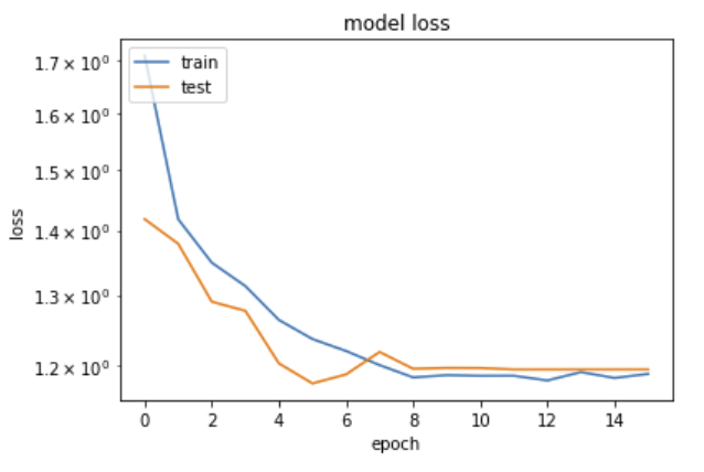
# plot training history
from matplotlib import pyplot as plt
plt.plot(history.history['loss'])
plt.plot(history.history['val_loss'])
plt.yscale('log')
plt.title('model loss')
plt.ylabel('loss')
plt.xlabel('epoch')
plt.legend(['train', 'test'], loc='upper left')
plt.show()


Using the test samples from the second file, one can produce the ROC curves and the confusion matrices as in the previous example.
Notebook #5
...
MLINFN-2
...
: lstm_btag.ipynb
The fifth notebook is very similar to the fourth, but uses a Long Short-Term Memory to input sequentially data instead of having a full matrix. The inputs are the same
...
