...
| Name | Institution | Mail Address | Social Contacts |
|---|---|---|---|
| Brunella D'Anzi | INFN Sezione di Bari | brunella.d'anzi@cern.ch | Skype: live:ary.d.anzi_1; Linkedin: brunella-d-anzi |
| Nicola De Filippis | INFN Sezione di Bari | nicola.defilippis@ba.infn.it | |
Domenico Diacono | INFN Sezione di Bari | domenico.diacono@ba.infn.it | |
| Walaa Elmetenawee | INFN Sezione di Bari | walaa.elmetenawee@cern.ch | |
| Giorgia Miniello | INFN Sezione di Bari | giorgia.miniello@ba.infn.it | |
| Andre Sznajder | Rio de Janeiro State University | sznajder.andre@gmail.com |
| Presentazione https://agenda.infn.it/event/26762/ |
|---|
How to Obtain Support
| brunella.d'anzi@cern.ch,giorgia.miniello@ba.infn.it | |
| Social | Skype: live:ary.d.anzi_1; Linkedin: brunella-d-anzi |
...
Particle Physics basic concepts: the Standard Model and the Higgs boson
...
The Standard Model of elementary particles represents our knowledge of the microscopic world. It describes the matter constituents (quarks and leptons) and their interactions (mediated by bosons), which are the electromagnetic, the weak, and the strong interactions.
...
# Plot of the metrics Efficiency x Purity -- ANN
# Looking at this curve we will choose a threshold on the ANN score
# for distinguishing between signal and background events
#plt.plot(t, p[:-1], label='purity_test')
#plt.plot(t_train, p_train[:-1], label='purity_train')
#plt.plot(t, r[:-1], label='efficiency_test')
#plt.plot(t_train, r_train[:-1], label='efficiency_test')
plt.rcParams['figure.figsize'] = (10,5)
plt.plot(t,p[:-1]*r[:-1],label='purity*efficiency_test')
plt.plot(t_train,p_train[:-1]*r_train[:-1],label='purity*efficiency_train')
plt.xlabel('Threshold/cut on the ANN score')
plt.ylabel('Purity*efficiency')
plt.title('Purity*efficiency vs Threshold on the ANN score',fontsize=12,fontweight='bold', color='r')
#plt.tick_params(width=2, grid_alpha=0.5)
plt.legend(markerscale=50)
plt.show()
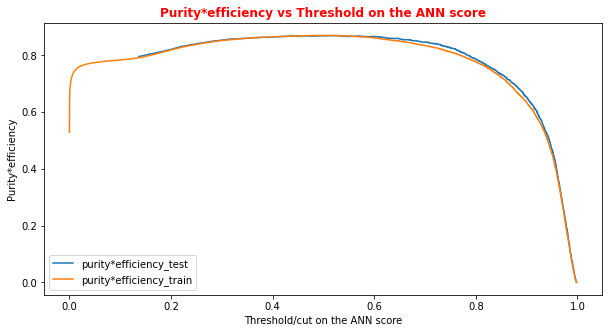
# Print metrics imposing a threshold for the test sample. In this way the student
# can use later the model's score to discriminate signal and bkg events for a fixing
# score

cut_dnn=0.6

# Transform predictions into a array of entries 0,1 depending if prediction is beyond the
# chosen threshold
y_pred = Y_prediction[:,0]
y_pred[y_pred >= cut_dnn]= 1 #classify them as signal
y_pred[y_pred < cut_dnn]= 0 #classify them as background
y_pred_train = Y_prediction_train[:,0]
y_pred_train[y_pred_train>=cut_dnn]=1
y_pred_train[y_pred_train<cut_dnn]=0

print("y_true.shape",y_true.shape)
print("y_pred.shape",y_pred.shape)
print("w_test.shape",w_test.shape)
print("Y_prediction",Y_prediction)
print("y_pred",y_pred)
...
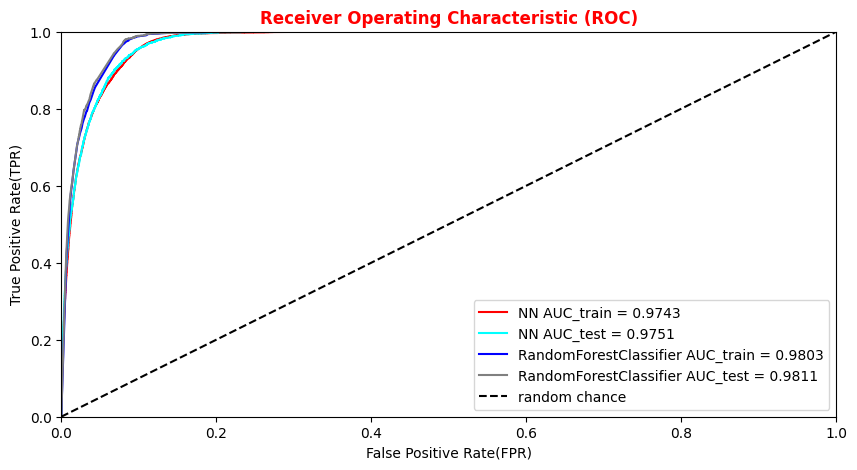
##Superimposition RF and ANN ROC curves
plt.rcParams['figure.figsize'] = (10,5)
plt.plot(fpr_train, tpr_train, color='red', label='NN AUC_train = %.4f' % (roc_auc_train))
plt.plot(fpr, tpr,  color='cyan', label='NN AUC_test = %.4f' % (roc_auc))
#Random Forest 1st method
plt.plot(fpr_train_rf,tpr_train_rf, color='blue', label='RandomForestClassifier AUC_train = %.4f' % (roc_auc_rf_train))
plt.plot(fpr_rf,tpr_rf, color='grey', label='RandomForestClassifier AUC_test = %.4f' % (roc_auc_rf))
#Random Forest 2nd method
#rfc_disp = plot_roc_curve(rfc, X_train_val,Y_train_val,color='brown',ax=ax, sample_weight=w_train )
#rfc_disp = plot_roc_curve(rfc, X_test, Y_test, color='grey',ax=ax, sample_weight=w_test)
#random chance
plt.plot([0, 1], [0, 1], linestyle='--', color='k', label='random chance')
plt.xlim([0, 1.0]) #fpr
plt.ylim([0, 1.0]) #tpr
plt.title('Receiver Operating Characteristic (ROC)',fontsize=12,fontweight='bold', color='r')
plt.xlabel('False Positive Rate(FPR)')
plt.ylabel('True Positive Rate(TPR)')
plt.legend(loc="lower right")
plt.show()
Plot physics observables
We can easily plot the quantities (e.g. ,
,
,
,
) for those events in the datasets which have the ANN and the RF output scores greater than the chosen decision threshold in order to show that the ML discriminators did learned from physics observables!
The subsections of this notebook part are:
...