| Table of Contents |
|---|
Author(s)
| Name | Institution | Mail Address | Social Contacts |
|---|---|---|---|
| Leonardo Giannini | INFN Sezione di Pisa / UCSD | leonardo.giannini@cern.ch | |
| Tommaso Boccali | INFN Sezione di Pisa | tommaso.boccali@pi.infn.it | Skype: tomboc73; Hangouts: tommaso.boccali@gmail.com |
How to Obtain Support
| tommaso.boccali@pi.infn.it, leonardo.giannini@cern.ch | |
| Social | Skype: tomboc73 |
| Jira |
General Information
| ML/DL Technologies | LSTM, CNN |
|---|---|
| Science Fields | High Energy Physics |
| Difficulty | Low |
| Language | English |
| Type | fully annotated and runnable |
...
| Info |
|---|
| Presentation made on : https://agenda.infn.it/event/25728/contributions/129752/attachments/78751/101917/go |
Software and Tools
| Programming Language | Python |
|---|---|
| ML Toolset | Keras + Tensorflow |
| Additional libraries | uproot |
| Suggested Environments | INFN-Cloud VM, bare Linux Node, Google CoLab |
Needed datasets
| Data Creator | CMS Experiment |
|---|---|
| Data Type | Simulation |
| Data Size | 1 GB |
| Data Source | INFN Pandora |
Short Description of the Use Case
Jets originating form b quarks have peculiar characteristics that one can exploit to discriminate them from jets originating from light quarks and gluons, and to better reconstruct their momentum. Both tasks have been dealt with using ML and are now tackled with Deep Learning techniques.
...
A complete explanation of the tutorial is available for download here.
How to execute it
Way #1: Use Googe Colab
Google's Colaboratory (https://colab.research.google.com/) is tool offered by Google which offers a Jupyter like environment on a Google hosted machine, with some added features, like the possibility to attach a GPU or a TPU if needed.
...
In the following the most important excerpts are described.
Way #2: Use Python from a ML-INFN Virtual machine
Another option is to use not Colab, but a real VM as made available by ML-INFN (LINK MISSING), or any properly configured host.
...
davix-get https://pandora.infn.it/public/307caa/dl/test93_0_20000.npz test93_0_20000.npz
davix-get https://pandora.infn.it/public/ec5e6a/dl/test93_20000_40000.npz test93_20000_40000.npz
Way #3: Use Jupyter notebooks from a ML-INFN Virtual machine
This way is somehow intermediate between #1 and #2. It still uses a browser environment and a Jupyter notebook, but the processing engine is on a ML-INFN instead of Google's public cloud.
You can get access to a Jupyter environment from XXX (same machine as #2), but insted from logging on that via ssh, you connect to hestname:888 and provide the password you selected at creation time. At than point, you can upload the .ipynb notebooks from drive-download-20200317T155726Z-001.zip.
Annotated Description
What is (jet) b-tagging?
It is the identification (or "tagging") of jets originating from bottom quark.
...
- Efficient and robust tracking needed
- Displaced tracks
- with good IP resolution
- Secondary vertex reconstruction
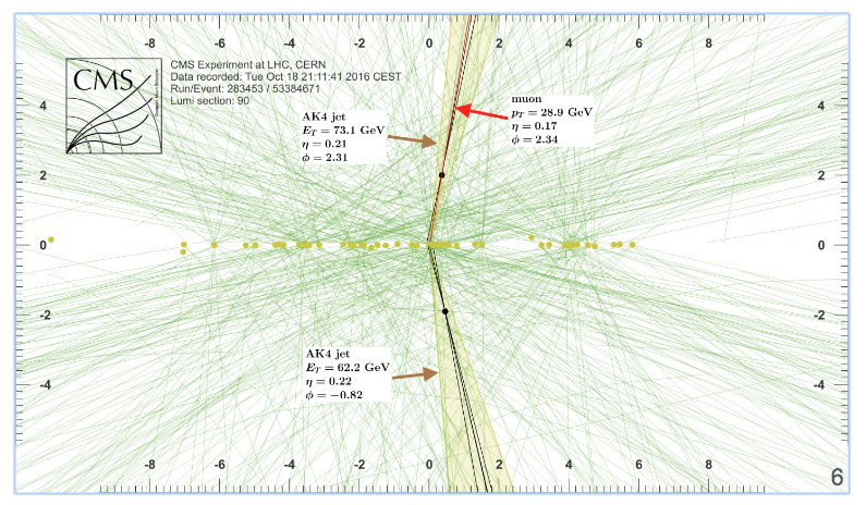
Typical b-tagging algorithms @ CMS
They
- Can use single discriminating variables
...
- 3 categories: vertex - no vertex - pseudovertex depending on the reconstruction of a secondary decay vertex;
- ~ 20 “tagging variables”, among which the parameters of a track subset, the presence of secondary vertices and leptons.
A new b-tagging algorithm
The rest of the tutorial focuses on the development of a "toy but realistic DNN algorithm", which includes vertexing, instead of having vertexing results as pre-computed input. Its inputs is, thus, mostly tracks. The real system, used by CMS, has better performance than the DeepCSV, with a (preliminary) ROC
...
Long-Short term memories (LSTM) are used in order to reduce the parameter count, since there is no reason to believe that any of the 20 tracks per "seed" should be treated differently. After the application of the LSTM, convolutional filters and dense layers are used to are used scale to 4 output classes ("b","c", "uds", "gluon").
The tutorial
The tutorial includes 5 Jupyter Notebooks, which can be run under Google's Colab. In order to be able and run and modify files, please use the link "Open in playground" as in the picture below, or generate a private copy of the notebook from the File menu.

Notebook #1: plot_NNinput.ipynb
This notebook loads a file containing precomputed features from MC events (from CMS), including reconstructed features and Monte Carlo Truth.
...
data relative to 20000 jets
- 52 variables per jet
Ntuple content kinematics
0. "jet_pt"
1. "jet_eta"
# of particles / vertices
2. "nCpfcand"
3. "nNpfcand",
4. "nsv",
5. "npv",
6. "n_seeds",
b tagging discriminataing variables
7. "TagVarCSV_trackSumJetEtRatio"
8. "TagVarCSV_trackSumJetDeltaR",
9. "TagVarCSV_vertexCategory",
10. "TagVarCSV_trackSip2dValAboveCharm",
11. "TagVarCSV_trackSip2dSigAboveCharm",
12. "TagVarCSV_trackSip3dValAboveCharm",
13. "TagVarCSV_trackSip3dSigAboveCharm",
14. "TagVarCSV_jetNSelectedTracks",
15. "TagVarCSV_jetNTracksEtaRel",
other kinematics
16. "jet_corr_pt",
17. "jet_phi",
18. "jet_mass",
19. detailed truth
19. "isB",
20. "isGBB",
21. "isBB",
...
41. "isPhysG",
42. "isPhysUndefined"
truth (6 categories)
43. "isB*1",
44. "isBB+isGBB",
45. "isLeptonicB+isLeptonicB_C",
46. "isC+isGCC+isCC",
47. "isUD+isS",
48. "isG*1",
49. "isUndefined*1",

truth as integer (used in the notebook)
50. "5x(isB+isBB+isGBB+isLeptonicB+isLeptonicB_C)+4x(isC+isGCC+isCC)+1x(isUD+isS)+21xisG+0xisUndefined",
alternative definition
51. "5x(isPhysB+isPhysBB+isPhysGBB+isPhysLeptonicB+isPhysLeptonicB_C)+4x(isPhysC+isPhysGCC+isPhysCC)+1x(isPhysUD+isPhysS)+21xisPhysG+0xisPhysUndefined"
...
isB=jetvars[:,-2]==5
isC=jetvars[:,-2]==4
isL=jetvars[:,-2]==1
isG=jetvars[:,-2]==21

categories=[isB, isC, isL, isG]
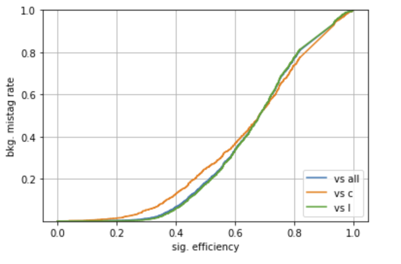
Plotting a ROC
A ROC curve can be constructed, using a scan on a specific input (use TagVarCSV_trackSip2dSigAboveCharm here), with the code
...
# b vs light and gluon roc curve
# B vs other categories -> we use isB


isBvsC = isB[isB+isC]
isBvsUSDG = isB[isB+isL+isG]

# B vs ALL roc curve

fpr, tpr, threshold = roc_curve(isB,jetvars[:,11])
auc1 = auc(fpr, tpr)

# B vs c

fpr2, tpr2, threshold = roc_curve(isBvsC,jetvars[:,11][isB+isC])
auc2 = auc(fpr2, tpr2)

# B vs light/gluon

fpr3, tpr3, threshold = roc_curve(isBvsUSDG, jetvars[:,11][isB+isL+isG])
auc3 = auc(fpr3, tpr3)

# print AUC

print (auc1, auc2, auc3)

pyplot.plot(tpr,fpr,label="vs all")
pyplot.plot(tpr2,fpr2,label="vs c")
pyplot.plot(tpr3,fpr3,label="vs l")
pyplot.xlabel("sig. efficiency")
pyplot.ylabel("bkg. mistag rate")
pyplot.ylim(0.000001,1)
pyplot.grid(True)
pyplot.legend(loc='lower right')
Notebook #2: plot_seedingTrackFeatures.ipynb
It is very similar to previous example, but looks into the other ntuples in the file, which we did not consider before
...
You can go on studying these features.
Notebook #3: keras_DNN.ipynb
This notebook trains a Dense network using the input features described in the previous sections.
...
Without cuts, a "b" is recognized 57% of the time as a "b" and 43% as a light. Clearly, this is low figure but depends on the cut on the output.
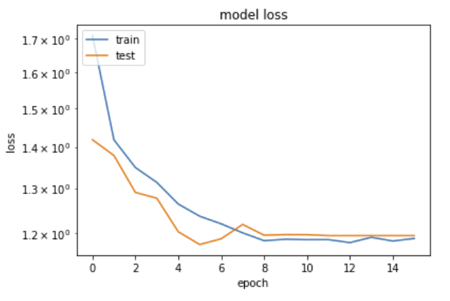
Notebook #4: CNN1x1_btag.ipynb
The fourth notebook builds a convolutional NN using the same input features, PLUS the single tracks features in arr_1
...
# train
history = model.fit([jetInfo, dataTRACKS], jetCategories, epochs=n_epochs, batch_size=batch_size, verbose = 2,
                validation_split=0.3,
                callbacks = [
                EarlyStopping(monitor='val_loss', patience=10, verbose=1),
                ReduceLROnPlateau(monitor='val_loss', factor=0.1, patience=2, verbose=1),
                TerminateOnNaN()])
# plot training history
from matplotlib import pyplot as plt
plt.plot(history.history['loss'])
plt.plot(history.history['val_loss'])
plt.yscale('log')
plt.title('model loss')
plt.ylabel('loss')
plt.xlabel('epoch')
plt.legend(['train', 'test'], loc='upper left')
plt.show()


Using the test samples from the second file, one can produce the ROC curves and the confusion matrices as in the previous example.
Notebook #5: lstm_btag.ipynb
The fifth notebook is very similar to the fourth, but uses a Long Short-Term Memory to input sequentially data instead of having a full matrix. The inputs are the same
...
From this point on, the treatment of the test samples, ROC, and confusion matrices are the same as in the previous example.
References
- Slides as presented at Scientific Data Analysis School at Scuola Normale, November 2019: here.
- CMS btagging results: here.
Attachments
| View file | ||||
|---|---|---|---|---|
|
| View file | ||||
|---|---|---|---|---|
|
| View file | ||||
|---|---|---|---|---|
|
...