...
You can get access to a Jupyter environment from XXX (same machine as #2), but insted instead from logging on that via ssh, you connect to hestname:888 8888 and provide the password you selected at creation time. At than point, you can upload the .ipynb notebooks from drive-download-20200317T155726Z-001.zip.
...
from matplotlib import pyplot as plt
plt.plot(history.history['loss'])
plt.plot(history.history['val_loss'])
plt.yscale('log')
plt.title('model loss')
plt.ylabel('loss')
plt.xlabel('epoch')
plt.legend(['train', 'test'], loc='upper left')
plt.show()
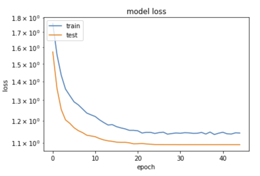
This is somehow counterintuitive with what we are usually taught: "loss will be lower on train than on validation samples, since the network tends to learn the specific quirks of a sample – this is usually called overtraining". Here we see the opposite, how can it be?
The solution comes from the fact that indeed, precisely in order to avoid overtraining, we have inserted in the network above Dropout layers. Their function is to randomly delete a fraction of the nodes and the connections, different in each training era, in order to "disturb" the convergence on the training sample. When processing on the validation sample, these nodes are not removed, and the performance on validation can indeed be better than on the (damaged on purpose) training sample.
We can use the second file as a validation set, to plot, for example, ROC curves. One builds a similar shaped set out of that
...