Name	Institution	Mail Address	Social Contacts
Brunella D'Anzi	INFN Sezione di Bari	brunella.d'anzi@cern.ch	Skype: live:ary.d.anzi_1; Linkedin: brunella-d-anzi
Nicola De Filippis	INFN Sezione di Bari	nicola.defilippis@ba.infn.it
Domenico Diacono	INFN Sezione di Bari	domenico.diacono@ba.infn.it
Walaa Elmetenawee	INFN Sezione di Bari	walaa.elmetenawee@cern.ch
Giorgia Miniello	INFN Sezione di Bari	giorgia.miniello@ba.infn.it
Andre Sznajder	Rio de Janeiro State University	sznajder.andre@gmail.com

Info
Presentation made on 26 Apr 2021 : https://agenda.infn.it/event/26762/

How to Obtain Support

Mail	brunella.d'anzi@cern.ch,giorgia.miniello@ba.infn.it
Social	Skype: live:ary.d.anzi_1; Linkedin: brunella-d-anzi

...

one that contains events distributed according to the null (in our case signal - there exist other conventions in actual physics analyses) hypothesis $H_{0}$ Image RemovedH₀ ;
another one according to the alternative (in our case background) hypothesis $H_{1}$ Image RemovedH₁ .

Then the algorithm must learn how to classify new datasets (the test dataset in our case).
This means that we have the same set of features (random variables) with their own distribution on the $H_{0}$ Image Removed and $H_{1}$ Image Removed hypothesesH₀ and H₁ hypotheses.

To obtain a good ML classifier with high discriminating power, we will follow the following steps:

...

Training (learning): a discriminator is built by using all the input variables. Then, the parameters are iteratively modified by comparing the discriminant output to the true label of the dataset (supervised machine learning algorithms, we will use two of them). This phase is crucial: one should tune the input variables and the parameters of the algorithm!
- As an alternative, algorithms that group and find patterns in the data according to the observed distribution of the input data are called unsupervised learning.
- A good habit is training multiple models with various hyperparameters on a “reduced” training set ( i.e. the full training set minus subtracting the so-called validation set), and then select the model that performs best on the validation set.
- Once, the validation process is over, you can re-train the best model on the full training set (including the validation set), and this gives you the final model.
Test: once the training has been performed, the discriminator score is computed in a separated, independent dataset for both $H_{0}$ Image Removed and $H_{1}$ Image RemovedH₀ and H₁ .
A comparison is made between test and training classifier and their performances (in terms of ROC curves) are evaluated.
- If the test fails and the performance of the test and training are different, this could be a symptom of overtraining and our model can be considered not good!

...

Particle Physics basic concepts: the Standard Model and the Higgs boson

...

Image Modified

The Standard Model of elementary particles represents our knowledge of the microscopic world. It describes the matter constituents (quarks and leptons) and their interactions (mediated by bosons), which are the electromagnetic, the weak, and the strong interactions.

...

Our physics problem consists in detecting the so-called “golden decay channel” channel” $H \to ZZ^{*} \to l^{+}l^{-}l'^{+}l'^{-}$ which is one of the possible Higgs boson's decays: its name is due to the fact that it has the clearest and cleanest signature of all the possible Higgs boson's decay modes. The decay chain is sketched here: the Higgs boson decays into Z boson pairs, which in turn decay into a lepton pair (in the picture, muon-antimuon or electron-positron pairs). In this exercise, we will use only datasets concerning the $4\mu$ Image Removed decay 4µ decay channel and the datasets about the 4e channel are given to you to be analyzed as an optional exercise. At the LHC experiments, the decay channel 2e2mu is also widely analyzed.

...

electrically-charged leptons (electrons or muons, denoted with $l$ Image Removedl)
particle jets (collimated streams of particles originating from quarks or gluons, denoted with $j$ Image Removedj).

For each object, several kinetic variables are measured:

the momentum transverse to the beam direction ( $pt$ Image Removedpt)
two angles $\theta$ Image Removed θ (polar) and $\phi$ Image Removed Φ (azimuthal) - see picture below for the CMS reference frame used.
for convenience, at hadron colliders, the pseudorapidity $\eta$ Image Removedη, defined as $\eta=-ln(tan(\eta/2))$ Image Removed is η=-ln(tan(η/2)) is used instead of the polar angle $\theta$ Image Removedθ.

We will use some of them for training our Machine Learning algorithms.

...

The notebook for this tutorial can be found here. The .ipynb file is available in the Attachment section and in this GitHub repository.

...

The datasets files are stored on Recas-Bari's ownCloud and are automatically loaded by the notebook. In case, they are also available here (four muons decay channel)for the main exercise and here (four electrons decay channel) for the optional exercise.

...

The first 2 columns contain information that is provided by experiments at the LHC that will not be used in the training of our Machine Learning algorithms, therefore we skip our explanation to the next columns.
The next variable is the f_weights. This corresponds to the probability of having that particular kind of physical process on the whole experiment. Indeed, it is a product of Branching Ratio (BR), geometrical acceptance and kinematic phase-space (generator level). It is very important for the training phase and you will use it later.
The variables f_massjj,f_deltajj,f_mass4l,f_Z1mass, and f_Z2mass are named high-level features (event features) since they contain overall information about the final-state particles (the mass of the two jets, their separation in space, the invariant mass of the four leptons, the masses of the two Z bosons). Note that the $m_{Z_{2}}$ Image Removed mass m_Z2 mass is lighter w.r.t. the $m_{Z_{1}}$ Image Removed onem_Z1 one. Why is that? In the Higgs boson production (hypothesis of mass = 125 GeV) only one of the Z bosons is an actual particle that has the nominal mass of 91.18 GeV. The other one is a virtual (off-mass shell) particle.
The other columns represent the low-level features (object kinematics observables), the basic measurements which are made by the detectors for the individual final state objects (in our case four charged leptons and jets) such as f_lept1(2,3,4)_pt(phi,eta) corresponding to their transverse momentum $pt$ Image Removed and pt and the spatial distribution of their tracks ( $\eta, \phi$ Image Removedη,Φ).

The same comments hold for the background datasets:

...

Question to students: Have a look to the parameter setting test_size. Why did we choose that small fraction of events to be used for the testing phase?

# Classical way to proceed, using a scikit-learn algorithm:

# X_train_val, X_test, Y_train_val , Y_test , W_train_val , W_test = 
# train_test_split(X, Y, W , test_size=0.2,shuffle=None,stratify=None )

# Alternative way, the one that we chose in order to study the model's performance 
# with ease (with an analogous procedure used by TMVA in ROOT framework)
# to keep information about the flag isSignal in both training and test steps. 

size= int(len(X[:,0]))
test_size = int(0.2*len(X[:,0]))
print('X (features) before splitting')
print('\n')
print(X.shape)
print('X (features) splitting between test and training')
X_test= X[0:test_size+1,:]
print('Test:')
print(X_test.shape)
X_train_val= X[test_size+1:len(X[:,0]),:]
print('Training:')
print(X_train_val.shape)
print('\n')
print('Y (target) before splitting')
print('\n')
print(Y.shape)
print('Y (target) splitting between test and training ')
Y_test= Y[0:test_size+1,:]
print('Test:')
print(Y_test.shape)
Y_train_val= Y[test_size+1:len(Y[:,0]),:]
print('Training:')
print(Y_train_val.shape)
print('\n')
print('W (weights) before splitting')
print('\n')
print(W.shape)
print('W (weights) splitting between test and training ')
W_test= W[0:test_size+1,:]
print('Test:')
print(W_test.shape)
W_train_val= W[test_size+1:len(W[:,0]),:]
print('Training:')
print(W_train_val.shape)
print('\n')

...

A Neural Networks (NN) can be classified according to the type of neuron interconnections and the flow of information.

Feed Forward Networks

Image Modified
A feedforward NN is a neural network where connections between the nodes do not form a cycle. In a feed-forward network information always moves one direction, from input to output, and it never goes backward. Feedforward NN can be viewed as mathematical models of a function $f: R^{N} \to R^{M}$ Image Modified.

Recurrent Neural Network

Image Modified
A Recurrent Neural Network (RNN) is the one that allows connections between nodes in the same layer, among each other or with previous layers.

Unlike feedforward neural networks, RNNs can use their internal state (memory) to process sequential input data.

...

Such a structure is also called Feedforward Multilayer Perceptron (MLP, see the picture).

Image Modified

The output of the $k_{th}$ Image Removed node k_th node of the $nth$ Image Removed layers n_th layers is computed as the weighted average of the input variables, with weights that are subject to optimization via training.

...

Then a bias or threshold parameter $w_{0}$ Image Removed is w₀ is applied. This bias accounts for the random noise, in the sense that it measures how well the model fits the training set (i.e. how much the model is able to correctly predict the known outputs of the training examples.) The output of a given node is: $y^{(n)}_{k}(\vec{x})=\phi (w^{n}_{0}\sum_{j=1}^{p^{(n)}}w^{(n)}_{kj}x_{j})$ .

...

During training we optimize the loss function, i.e. reduce the error between actual and predicted values. Since we deal with a binary classification problem, the $y_{true}$ Image Removed can y_true can take on just two values, $y_{true} =0$ Image Removed y_true = 0 (for hypothesis $H_{0}$ Image RemovedH₁) and $y_{true} = 1$ Image Removed = 1 (for hypothesis $H_{1}$ Image RemovedH₀).

A popular algorithm to optimize the weights consists of iteratively modifying the weights after each training observation or after a bunch of training observations by doing a minimization of the loss function.

...

Layers are the basic building blocks of neural networks in Keras. A layer consists of a tensor-in tensor-out computation function (the layer's call method) and some state, held in TensorFlow variables (the layer's weights).

Callbacks API

Image Modified

A callback is an object that can perform actions at various stages of training (e.g. at the start or end of an epoch, before or after a single batch, etc).

...

Regularization layers : the dropout layer

Image Modified

The Dropout layer randomly sets input units to 0 with a frequency of rate at each step during training time, which helps prevent overtraining. Inputs not set to 0 are scaled up by 1/(1-rate) such that the sum over all inputs is unchanged.

Note that the Dropout layer only applies when training is set to True such that no values are dropped during inference. When using model.fit, training will be appropriately set to Trueautomatically, and in other contexts, you can set the flag explicitly to True when calling the layer.

Artificial Neural Network implementation

We can now start to define the first architecture. The most simple approach is using fully connected layers (Dense layers in Keras/Tensorflow), with seluactivation function and a sigmoid final layer, since we are affording a binary classification problem.

...

the assignment of a terminal node to a class;
the stop splitting of the single tree;
selection criteria of splits.

...

Grid Search for Parameter estimation

A machine learning model has two types of parameters. The first type are is the parameters that are learned through a machine learning model while the second type are the hyperparameters whose value is used to control the learning process.

...

First, we introduce the terms positive and negative referring to the classifier’s prediction, and the terms true and false referring to whether the network prediction corresponds to the observation (the "truth" level). In our Higgs boson binary classification exercise, we can think the negative outcome as the one labeling background (that, in the last sigmoid layer of our network, would mean a number close to 0 - in the Random Forest score would mean a number equals to zero), and the positive outcome the outcome as the one labeling signal (that, in the last sigmoid layer of our network, would mean a number close to 1 - random forest score equals to zero).

...

# Plot of the metrics Efficiency x Purity -- ANN 
# Looking at this curve we will choose a threshold on the ANN score
# for distinguishing between signal and background events
#plt.plot(t, p[:-1], label='purity_test')
#plt.plot(t_train, p_train[:-1], label='purity_train')
#plt.plot(t, r[:-1], label='efficiency_test')
#plt.plot(t_train, r_train[:-1], label='efficiency_test')
plt.rcParams['figure.figsize'] = (10,5)
plt.plot(t,p[:-1]*r[:-1],label='purity*efficiency_test')
plt.plot(t_train,p_train[:-1]*r_train[:-1],label='purity*efficiency_train')
plt.xlabel('Threshold/cut on the ANN score')
plt.ylabel('Purity*efficiency')
plt.title('Purity*efficiency vs Threshold on the ANN score',fontsize=12,fontweight='bold', color='r')
#plt.tick_params(width=2, grid_alpha=0.5)
plt.legend(markerscale=50)
plt.show()

Image Modified

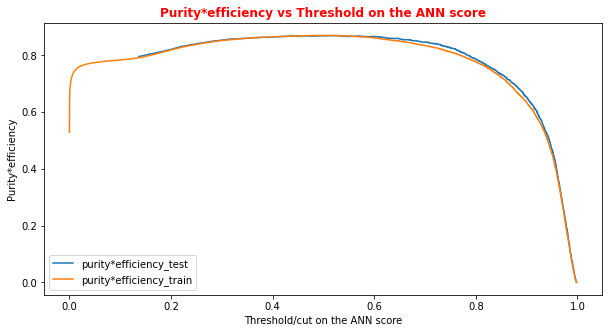
# Print metrics imposing a threshold for the test sample. In this way the student
# can use later the model's score to discriminate signal and bkg events for a fixing
# score

cut_dnn=0.6

# Transform predictions into a array of entries 0,1 depending if prediction is beyond the
# chosen threshold
y_pred = Y_prediction[:,0] 
y_pred[y_pred >= cut_dnn]= 1 #classify them as signal
y_pred[y_pred < cut_dnn]= 0 #classify them as background
y_pred_train = Y_prediction_train[:,0]
y_pred_train[y_pred_train>=cut_dnn]=1
y_pred_train[y_pred_train<cut_dnn]=0

print("y_true.shape",y_true.shape)
print("y_pred.shape",y_pred.shape)
print("w_test.shape",w_test.shape)
print("Y_prediction",Y_prediction)
print("y_pred",y_pred)

...

Cut/Threshold on the ANN output : 0.6000 

Confusion matrix ANN
Image Removed

Image Added

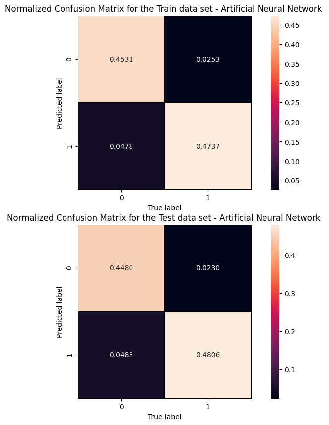
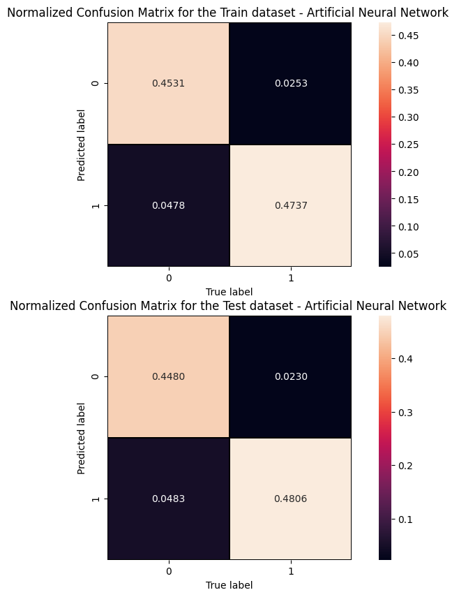
An alternative way to check overfitting, and choosing correctly a threshold for selecting signal events, is plotting signal and background ANN predictions for the training and test datasets. If the distributions are quite similar it means that the algorithm learned how to generalize!
For measuring quantitatively the overfitting one can perform a Kolmogorov-Smirnov test that we will not implement here.

...

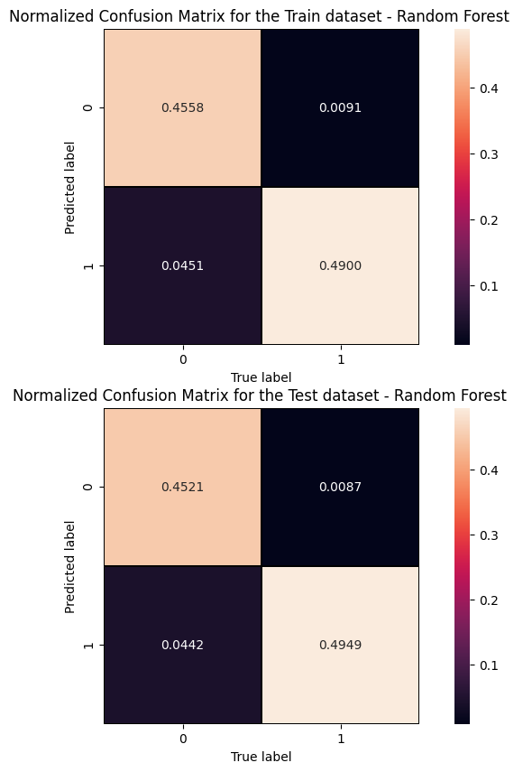
Cut/Threshold on the Random Forest output : 0.6000

Image RemovedImage Added

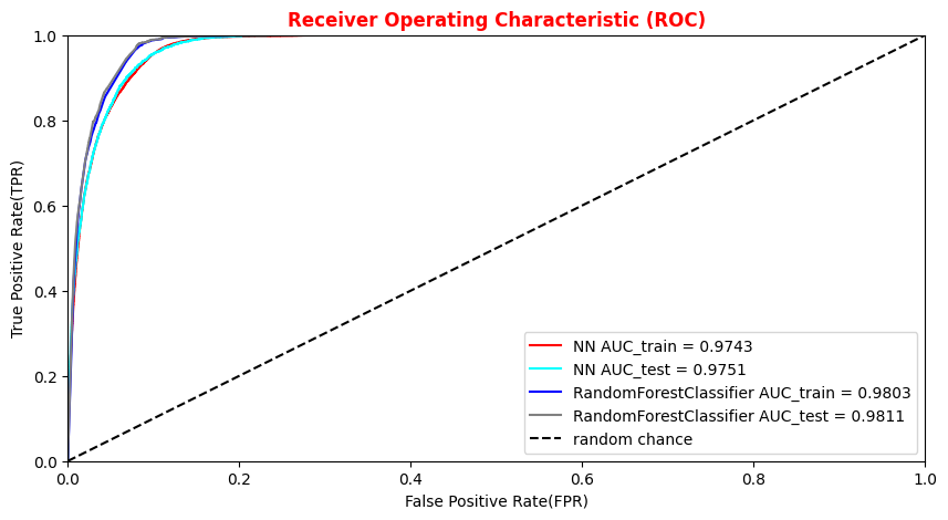
##Superimposition RF and ANN ROC curves
plt.rcParams['figure.figsize'] = (10,5)
plt.plot(fpr_train, tpr_train, color='red', label='NN AUC_train = %.4f' % (roc_auc_train))
plt.plot(fpr, tpr,  color='cyan', label='NN AUC_test = %.4f' % (roc_auc))
#Random Forest 1st method
plt.plot(fpr_train_rf,tpr_train_rf, color='blue', label='RandomForestClassifier AUC_train = %.4f' % (roc_auc_rf_train))
plt.plot(fpr_rf,tpr_rf, color='grey', label='RandomForestClassifier AUC_test = %.4f' % (roc_auc_rf))
#Random Forest 2nd method
#rfc_disp = plot_roc_curve(rfc, X_train_val,Y_train_val,color='brown',ax=ax, sample_weight=w_train )
#rfc_disp = plot_roc_curve(rfc, X_test, Y_test, color='grey',ax=ax, sample_weight=w_test)
#random chance
plt.plot([0, 1], [0, 1], linestyle='--', color='k', label='random chance')
plt.xlim([0, 1.0]) #fpr
plt.ylim([0, 1.0]) #tpr
plt.title('Receiver Operating Characteristic (ROC)',fontsize=12,fontweight='bold', color='r')
plt.xlabel('False Positive Rate(FPR)')
plt.ylabel('True Positive Rate(TPR)')
plt.legend(loc="lower right")
plt.show()

Image Modified

Plot physics observables

We can easily plot the quantities (e.g. $m_{jj}$ , $\eta_{j}$ , $m_{4l}$ , $m_{Z_{1}}$ , $m_{Z_{2}}$ ) for those events in the datasets which have the ANN and the RF output scores greater than the chosen decision threshold in order to show that the ML discriminators did learned from physics observables!
The subsections of this notebook part are:

...

Question to students: What happens if you switch to the $4e$ Image Removed decay 4e decay channel? You can submit your model (see the ML challenge below) for this physical process as well!

...

You can participate as a single participant or as a team
The winner is the one scoring the best AUC in the challenge samples!
In the next box, you will find some lines of code for preparing an output csv file, containing your y_predic for this new dataset!
Choose a meaningful name for your result csv file (i.e. your name, or your team name, the model used for the training phase, and the decay channel - 4 $\mu$ Image Removed or 4 $e$ Image Removed 4μ or 4e - but avoid to submit results.csv)
Download the csv file and upload it here: https://recascloud.ba.infn.it/index.php/s/CnoZuNrlr3x7uPI
You can submit multiple results, paying attention to name them accordingly (add the version number, such as v1, v34, etc.)
You can use this exercise as a starting point (train over constituents)
We will consider your best result for the final score.
The winner will be asked to present the ML architecture!

...

(164560, 5)
(164560, 1)
[[1.7398037e-05]
 [3.2408145e-01]
 [1.1487612e-04]
 ...
 [2.4130943e-01]
 [1.4921818e-05]
 [8.3920550e-01]]

Out[ ]

	0
0	1.739804e-05
1	3.240815e-01
2	1.148761e-04
3	6.713818e-10
4	4.403101e-01

...

https://recascloud.ba.infn.it/index.php/s/CnoZuNrlr3x7uPI

References

Attachments

Here it is the complete notebook:

View file

name	VBF_H_4l_ML_exercise.ipynb
height	250

Space shortcuts

Page tree

Versions Compared

Old Version 112

New Version Current

Key

How to Obtain Support

Particle Physics basic concepts: the Standard Model and the Higgs boson

Image Modified

Feed Forward Networks

Recurrent Neural Network

Callbacks API

Regularization layers : the dropout layer

Artificial Neural Network implementation

Grid Search for Parameter estimation

Image Modified

Image Modified

Plot physics observables

References

Attachments

Space shortcuts

Page tree

Page History

Versions Compared

Old Version 112

New Version Current

Key

How to Obtain Support

Particle Physics basic concepts: the Standard Model and the Higgs boson

Image Modified

Feed Forward Networks

Recurrent Neural Network

Callbacks API

Regularization layers : the dropout layer

Artificial Neural Network implementation

Grid Search for Parameter estimation

Image Modified

Image Modified

Plot physics observables

References

Attachments