...
X (features) before splitting


(114984, 5)
X (features) splitting between test and training
Test:
(22997, 5)
Training:
(91987, 5)


Y (target) before splitting


(114984, 1)
Y (target) splitting between test and training
Test:
(22997, 1)
Training:
(91987, 1)


W (weights) before splitting


(114984, 1)
W (weights) splitting between test and training
Test:
(22997, 1)
Training:
(91987, 1)
Description of the Artificial Neural Network (ANN) model and KERAS API
In this section you will find the following subsections:
...
Note that the Dropout layer only applies when training is set to True such that no values are dropped during inference. When using model.fit, training will be appropriately set to Trueautomatically, and in other contexts, you can set the kwarg explicitly to True when calling the layer.
Artificial Neural Network implementation
We can now start to define a first architecture. The most simple approach is using fully connected layers (Dense layers in Keras/Tensorflow), with seluactivation function and a sigmoid final layer, since we are affording a binary classification problem.
...
To avoid overfitting we use also Dropout layers and some callback functions.
# Define Neural Network with 3 hidden layers ( #h1=10*NINPUT , #h2=2*NINPUT , #h3=NINPUT ) & Dropout layers

input  = Input(shape=(NINPUT,), name = 'input')
hidden = Dense(NINPUT*10, name = 'hidden1', kernel_initializer='normal', activation='selu')(input)
hidden = Dropout(rate=0.1)(hidden)
hidden = Dense(NINPUT*2 , name = 'hidden2', kernel_initializer='normal', activation='selu')(hidden)
hidden = Dropout(rate=0.1)(hidden)
hidden = Dense(NINPUT, name = 'hidden3', kernel_initializer='normal', activation='selu')(hidden)
hidden = Dropout(rate=0.1)(hidden)
output  = Dense(1 , name = 'output', kernel_initializer='normal', activation='sigmoid')(hidden)


# create the model
model = Model(inputs=input, outputs=output)
# Define the optimizer ( minimization algorithm )
#optim = SGD(lr=0.01,decay=1e-6)
#optim = Adam( lr=0.0001 )
#optim = Adagrad(learning_rate=0.0001 )
#optim = Adadelta(learning_rate=0.0001 )
#optim = RMSprop() #default lr= 1e-3
optim = RMSprop(lr = 1e-4)

# print learning rate each epoch to see if reduce_LR is working as expected

def get_lr_metric(optim):
    def lr(y_true, y_pred):
        return optim.lr
    return lr

# compile the model
#model.compile(optimizer=optim, loss='mean_squared_error', metrics=['accuracy'], weighted_metrics=['accuracy'])
#model.compile(optimizer=optim, loss='mean_squared_error', metrics=['accuracy'])
model.compile( optimizer=optim, loss='binary_crossentropy', metrics=['accuracy'], weighted_metrics=['accuracy'])
#accuracy (defined as the number of good matches between the predictions and the class labels)
# print the model summary
model.summary()
Model: "model"
_________________________________________________________________
Layer (type)                 Output Shape              Param #
=================================================================
input (InputLayer)           [(None, 5)]               0
_________________________________________________________________
hidden1 (Dense)              (None, 50)                300
_________________________________________________________________
dropout (Dropout)            (None, 50)                0
_________________________________________________________________
hidden2 (Dense)              (None, 10)                510
_________________________________________________________________
dropout_1 (Dropout)          (None, 10)                0
_________________________________________________________________
hidden3 (Dense)              (None, 5)                 55
_________________________________________________________________
dropout_2 (Dropout)          (None, 5)                 0
_________________________________________________________________
output (Dense)               (None, 1)                 6
=================================================================
Total params: 871
Trainable params: 871
Non-trainable params: 0
_________________________________________________________________plot_model(model, show_shapes=True, show_layer_names=True)
# The student can have his/her model saved:
model_file = 'ANN_model.h5'

##Call functions implementation to monitor the chosen metrics
checkpoint = keras.callbacks.ModelCheckpoint(filepath = model_file,
                                             monitor = 'val_loss',
                                             mode='min',
                                             save_best_only = True)

#Stop training when a monitored metric has stopped improving
early_stop = keras.callbacks.EarlyStopping(monitor = 'val_loss',
                                           mode='min',# quantity that has to be monitored(to be minimized in this case)
                              patience = 50, # Number of epochs with no improvement after which training will be stopped.
                              min_delta = 1e-7,
                              restore_best_weights = True) # update the model with the best-seen weights

#Reduce learning rate when a metric has stopped improving
reduce_LR = keras.callbacks.ReduceLROnPlateau( monitor = 'val_loss',
                                              mode='min',# quantity that has to be monitored
                                              min_delta=1e-7,
                                              factor = 0.1, # factor by which LR has to be reduced...
                                              patience = 10, #...after waiting this number of epochs with no improvements
                                              #on monitored quantity
                                              min_lr= 0.00001 )


callback_list = [reduce_LR, early_stop, checkpoint]
#callback_list = [checkpoint]
#callback_list = [ early_stop, checkpoint]
# Number of training epochs
# nepochs=500
nepochs=200
# Batch size
batch=250
# Train classifier (2 minutes more or less)
history = model.fit(X_train_val[:,0:NINPUT],
                    Y_train_val,
                    epochs=nepochs,
                    sample_weight=W_train_val,
                    batch_size=batch,
                    callbacks = callback_list,
                    verbose=1, # switch to 1 for more verbosity
                    validation_split=0.3 ) # fix the validation dataset size
model = keras.models.load_model('ANN_model.h5')
Description of the Random Forest (RF) and Scikit-learn library
In this section you will find the following subsections:
- Introduction to the Random Forest algorithm
If you have the knowledge about RF you may skip it. - Optional exercise: draw a decision tree
Here you find an atypical exercise in which it is suggested to think about the growth of a decision tree in this specific physics problem.
What is Scikit-learn library?
Scikit-learn is a simple and efficient tools for predictive data analysis,accessible to everybody, and reusable in various contexts. It is built on NumPy, SciPy, and matplotlib scientific libraries.
Introduction to the Random Forest algorithm
Decision Trees and their extension Random Forests are robust and easy-to-interpret machine learning algorithms for Classification tasks.
Decision Trees comprise a simple and fast way of learning a function that maps data x to outputs y, where x can be a mix of categorical and numeric variables and y can be categorical for classification, or numeric for regression.
Comparison with Neural Networks
(Deep) Neural Networks pretty much do the same thing. However, despite their power against larger and more complex data sets, they are extremely hard to interpret and they can take many iterations and hyperparameter adjustments before a good result is had.
One of the biggest advantages of using Decision Trees and Random Forests is the ease in which we can see what features or variables contribute to the classification or regression and their relative importance based on their location depthwise in the tree.
Decision Tree
A decision tree is a sequence of selection cuts that are applied in a specified order on a given variable data sets.
Each cut splits the sample into nodes, each of which corresponds to a given number of observations classified as class1 (signal) or as class2 (background).
A node may be further split by the application of the subsequent cut in the tree.Nodes in which either signal or background is largely dominant are classified as leafs, and no further selection is applied.
A node may also be classified as leaf, and the selection path is stopped, in case too few observations per node remain, or in case the total number of identified nodes is too large, and different criteria have been proposed and applied in real implementations.
Each branch on a tree represents one sequence of cuts. Along the decision tree, the same variable may appear multiple times, depending on the depth of the tree, each time with a different applied cut, possibly even with different inequality directions.
Selection cuts can be tuned in order to achieve the best split level in each node according to some metrics (gini index, cross entropy...). Most of them are related to the purity of a node, that is the fraction of signal events over the whole events set in a given node P=S/(S+B).
The gain due to the splitting of a node A into the nodes B1 and B2, which depends on the chosen cut, is given by: , where I denotes the adopted metric (G or E, in case of the Gini index or cross entropy introduced above). By varying the cut, the optimal gain may be achieved.
Pruning Tree
A solution to the overtraining is pruning, that is eliminating subtrees (branches) that seem too specific to training sample:
- a node and all its descendants turn into a leaf
- stop tree growth during building phase
Be Careful: early stopping condition may prevent from discovering further useful splitting. Therefore, grow the full tree and when result from subtrees are not significantly different from result of the parent one, prune them!
From tree to the forest
The random forest algorithm consists of ‘growing’ a large number of individual decision trees that operate as an ensemble from replicas of the training samples obtained by randomly resampling the input data (features and examples). 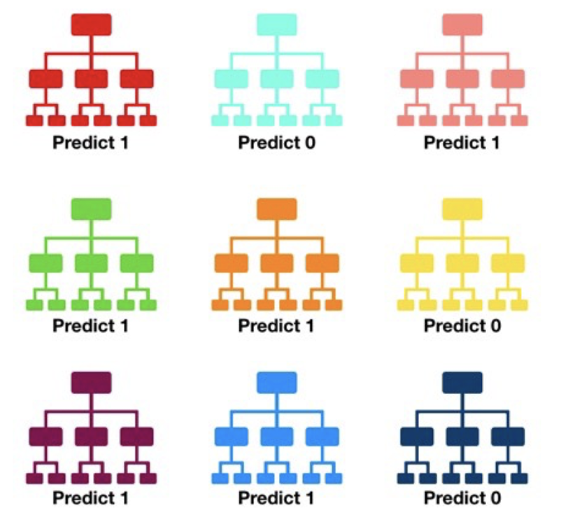
Its main characteristics are:
No minimum size is required for leaf nodes. The final score of the algorithm is given by an unweighted average of the prediction (zero or one) by each individual tree.
Each individual tree in the random forest splits out a class prediction and the class with the most votes becomes our model’s prediction.
As a large number of relatively uncorrelated models (trees) operating as a committee,this algorithm will outperform any of the individual constituent models. The reason for this wonderful effect is that the trees protect each other from their individual errors (as long as they don’t constantly all err in the same direction). While some trees may be wrong, many other trees will be right, so as a group the trees are able to move in the correct direction.
In a single decision tree, we consider every possible feature and pick the one that produces the best separation between the observations in the left node vs. those in the right node. In contrast, each tree in a random forest can pick only from a random subset of features (bagging).This forces even more variation amongst the trees in the model and ultimately results in lower correlation across trees and more diversification.
Feature importance
The relative rank (i.e. depth) of a feature used as a decision node in a tree can be used to assess the relative importance of that feature with respect to the predictability of the target variable. Features used at the top of the tree contribute to the final prediction decision of a larger fraction of the input samples. The expected fraction of the samples they contribute to can thus be used as an estimate of the relative importance of the features. In scikit-learn, the fraction of samples a feature contributes to is combined with the decrease in impurity from splitting them to create a normalized estimate of the predictive power of that feature.
Warning: The impurity-based feature importances computed on tree-based models suffer from two flaws that can lead to misleading conclusions:
- They are computed on statistics derived from the training dataset and therefore do not necessarily inform us on which features are most important to make good predictions on held-out dataset.
- They favor high cardinality features, that is features with many unique values. Permutation feature importance is an alternative to impurity-based feature importance that does not suffer from these flaws.
For this complexity we will not use show it in this exercise. Learn more here.
Optional exercise : Draw a decision tree
Here you are an example of how you can build a decision tree by yourself ! Try to imagine how the decision tree's growth could proceed in our analysis case and complete it! We give you some hints!