...
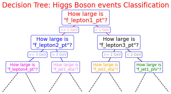
import matplotlib.pyplot as plt
%matplotlib inline
fig = plt.figure(figsize=(10, 4))
ax = fig.add_axes([0, 0, 0.8, 1], frameon=False, xticks=[], yticks=[])
ax.set_title('Decision Tree: Higgs Boson events Classification', size=24,color='red')

def text(ax, x, y, t, size=20, **kwargs):
    ax.text(x, y, t,
            ha='center', va='center', size=size,
            bbox=dict( boxstyle='round', ec='blue', fc='w' ), **kwargs)

# Here you are the variables we can use for the training phase:
# --------------------------------------------------------------------------
# High level features:
# ['f_massjj', 'f_deltajj', 'f_mass4l', 'f_Z1mass' , 'f_Z2mass']
# --------------------------------------------------------------------------
# Low level features:
#        [ 'f_lept1_pt','f_lept1_eta','f_lept1_phi', \
#          'f_lept2_pt','f_lept2_eta','f_lept2_phi', \
#          'f_lept3_pt','f_lept3_eta','f_lept3_phi', \
#          'f_lept4_pt','f_lept4_eta','f_lept4_phi', \
#          'f_jet1_pt','f_jet1_eta','f_jet1_phi', \
#          'f_jet2_pt','f_jet2_eta','f_jet2_phi']
#---------------------------------------------------------------------------
text(ax, 0.5, 0.9, "How large is\n\"f_lepton1_pt\"?", 20,color='red')
text(ax, 0.3, 0.6, "How large is\n\"f_lepton2_pt\"?", 18,color='blue')
text(ax, 0.7, 0.6, "How large is\n\"f_lepton3_pt\"?", 18)
text(ax, 0.12, 0.3, "How large is\n\"f_lepton4_pt\"?", 14,color='magenta')
text(ax, 0.38, 0.3, "How large is\n\"f_jet1_eta\"?", 14,color='violet')
text(ax, 0.62, 0.3, "How large is\n\"f_jet2_eta\"?", 14,color='orange')
text(ax, 0.88, 0.3, "How large is\n\"f_jet1_phi\"?", 14,color='green')

text(ax, 0.4, 0.75, ">= 1 GeV", 12, alpha=0.4,color='red')
text(ax, 0.6, 0.75, "< 1 GeV", 12, alpha=0.4,color='red')

text(ax, 0.21, 0.45, ">= 3 GeV", 12, alpha=0.4,color='blue')
text(ax, 0.34, 0.45, "< 3 GeV", 12, alpha=0.4,color='blue')

text(ax, 0.66, 0.45, ">= 2 GeV", 12, alpha=0.4,color='black')
text(ax, 0.79, 0.45, "< 2 GeV", 12, alpha=0.4,color='black')

ax.plot([0.3, 0.5, 0.7], [0.6, 0.9, 0.6], '-k',color='red')
ax.plot([0.12, 0.3, 0.38], [0.3, 0.6, 0.3], '-k',color='blue')
ax.plot([0.62, 0.7, 0.88], [0.3, 0.6, 0.3], '-k')
ax.plot([0.0, 0.12, 0.20], [0.0, 0.3, 0.0], '--k')
ax.plot([0.28, 0.38, 0.48], [0.0, 0.3, 0.0], '--k')
ax.plot([0.52, 0.62, 0.72], [0.0, 0.3, 0.0], '--k')
ax.plot([0.8, 0.88, 1.0], [0.0, 0.3, 0.0], '--k')
ax.axis([0, 1, 0, 1])

fig.savefig('05.08-decision-tree.png')
Random Forest implementation
Now you can start to define a second ML architecture setting the tree construction parameters to fix:
- the assignment of a terminal node to a class;
- the stop splitting of the single tree;
- selection criteria of splits.
Grid Search for Parameter estimation
A machine learning model has two types of parameters. The first type of parameters is the parameters that are learned through a machine learning model while the second type of parameters are the hyper parameter that we pass to the machine learning model.
Normally we set the value for these hyper parameters by hand, as we did for our ANN, and see what parameters result in the best performance. However, randomly selecting the parameters for the algorithm can be exhaustive.
Also, it is not easy to compare the performance of different algorithms by randomly setting the hyper parameters because one algorithm may perform better than the other with a different set of parameters. And if the parameters are changed, the algorithm may perform worse than the other algorithms.
Therefore, instead of randomly selecting the values of the parameters, a better approach would be to develop an algorithm that automatically finds the best parameters for a particular model. Grid Search is one such algorithm.
from sklearn.ensemble import RandomForestClassifier
from sklearn.metrics import plot_roc_curve
from sklearn.model_selection import GridSearchCV
Let's implement the grid search algorithm for our Random Forest discriminator!
Grid Search algorithm basically tries all possible combinations of parameter values and returns the combination with the highest accuracy. The Grid Search algorithm can be very slow, owing to the potentially huge number of combinations to test. Furthermore, the cross-validation further increases the execution!
For these reasons, the algorithm is commented in the following code cells and images of the outputs are left to you!
To read more about cross-validation on Scikit-learn:
Cross_validation
To read more about GridSearchCV algorithm on Scikit-learn:
#classifier = RandomForestClassifier(random_state=7)# The first step we need to perform is to # create a dictionary of all the parameters and their corresponding # set of values that you want to test for best performance. # The name of the dictionary items corresponds to the parameter name # and the value corresponds to the list of values for the parameter. # The parameter values that we want to try out # are passed in the list. In the below code we want to find # which values of the RF hyperparameters provides the highest accuracy #grid_param = { # 'criterion': ['gini','entropy'], # 'n_estimators': [300, 500], # 'bootstrap': [True, False], # 'max_depth': [3,5], # 'min_samples_leaf':[300,500], # 'min_samples_split':[200,400], # 'max_features':[3,4,5] # }
# Once the parameter dictionary is created,
# the next step is to create an instance of the GridSearchCV class.
# You need to pass values for the estimator parameter,
# which basically is the algorithm that you want to execute.
# The param_grid parameter takes the parameter dictionary that we
# just created as parameter, the scoring parameter takes the performance metrics,
# the cv parameter corresponds to number of folds,
# which is 5 in our case, and finally the n_jobs parameter refers to the
# number of CPU's that you want to use for execution.
# A value of -1 for n_jobs parameter means that use all available computing power.
# This can be handy if you have large number amount of data.

#gd_sr = GridSearchCV(estimator=classifier,
#                     param_grid=grid_param, #parameter dictionary
#                     scoring='accuracy', #performance metrics
#                     cv=3, #number of folds
#                     n_jobs=-1) #use all available computing power
# Time required : 7h 50 minutes
# gd_sr.fit(X_train_val, np.ravel(Y_train_val))
Output of the previous code cell:
#best_parameters = gd_sr.best_params_
#print('Best parameters:')
#print(best_parameters)
#best_result = gd_sr.best_score_
#print('Best metrics score (accuracy):')
#print(best_result)
Output of the previous code cell: