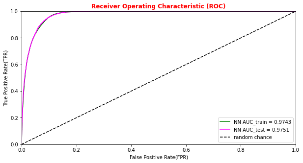
...

# Plotting the ANN ROC curve on the test and training datasets
roc_auc = auc(fpr, tpr)
roc_auc_train = auc(fpr_train,tpr_train)
plt.rcParams['figure.figsize'] = (10,5)
plt.plot(fpr_train, tpr_train,  color='green', label='NN AUC_train = %.4f' % (roc_auc_train))
plt.plot(fpr, tpr, color='magenta', label='NN AUC_test = %.4f' % (roc_auc))
# Comparison with the random chance curve
plt.plot([0, 1], [0, 1], linestyle='--', color='k', label='random chance')
plt.xlim([0, 1.0]) #fpr
plt.ylim([0, 1.0]) #tpr
plt.xlabel('False Positive Rate(FPR)')
plt.ylabel('True Positive Rate(TPR)')
plt.title('Receiver Operating Characteristic (ROC)',fontsize=12,fontweight='bold', color='r')
plt.legend(loc="lower right")
plt.show()

Image Added

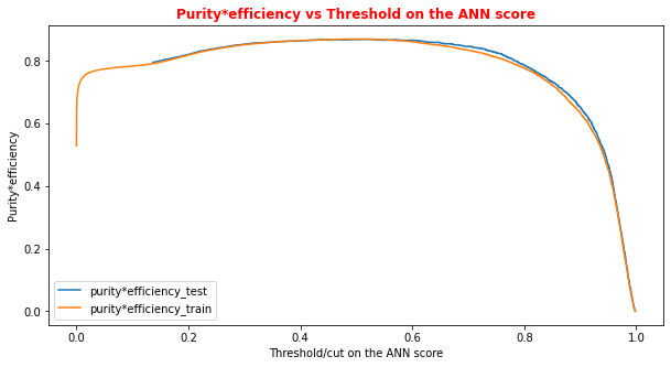
# Plot of the metrics Efficiency x Purity -- ANN 
# Looking at this curve we will choose a threshold on the ANN score
# for distinguishing between signal and background events
#plt.plot(t, p[:-1], label='purity_test')
#plt.plot(t_train, p_train[:-1], label='purity_train')
#plt.plot(t, r[:-1], label='efficiency_test')
#plt.plot(t_train, r_train[:-1], label='efficiency_test')
plt.rcParams['figure.figsize'] = (10,5)
plt.plot(t,p[:-1]*r[:-1],label='purity*efficiency_test')
plt.plot(t_train,p_train[:-1]*r_train[:-1],label='purity*efficiency_train')
plt.xlabel('Threshold/cut on the ANN score')
plt.ylabel('Purity*efficiency')
plt.title('Purity*efficiency vs Threshold on the ANN score',fontsize=12,fontweight='bold', color='r')
#plt.tick_params(width=2, grid_alpha=0.5)
plt.legend(markerscale=50)
plt.show()

Image Added

# Print metrics imposing a threshold for the test sample. In this way the student
# can use later the model's score to discriminate signal and bkg events for a fixing
# score

cut_dnn=0.6

# Transform predictions into a array of entries 0,1 depending if prediction is beyond the
# chosen threshold
y_pred = Y_prediction[:,0] 
y_pred[y_pred >= cut_dnn]= 1 #classify them as signal
y_pred[y_pred < cut_dnn]= 0 #classify them as background
y_pred_train = Y_prediction_train[:,0]
y_pred_train[y_pred_train>=cut_dnn]=1
y_pred_train[y_pred_train<cut_dnn]=0

print("y_true.shape",y_true.shape)
print("y_pred.shape",y_pred.shape)
print("w_test.shape",w_test.shape)
print("Y_prediction",Y_prediction)
print("y_pred",y_pred)

y_true.shape (22997,)
y_pred.shape (22997,)
w_test.shape (22997,)
Y_prediction [[1.]
 [1.]
 [0.]
 ...
 [0.]
 [1.]
 [0.]]
y_pred [1. 1. 0. ... 0. 1. 0.]

# Other Metrics values for the ANN algorithm having fixed an ANN score threshold
accuracy  = accuracy_score(y_true, y_pred, sample_weight=w_test)
precision = precision_score(y_true, y_pred, sample_weight=w_test)
recall    = recall_score(y_true, y_pred, sample_weight=w_test)
f1 = 2*precision*recall/(precision+recall)
cm = confusion_matrix( y_true, y_pred, sample_weight=w_test)
print('Cut/Threshold on the ANN output : %.4f' % cut_dnn)
print('ANN Test Accuracy: %.4f' % accuracy)
print('ANN Test Precision/Purity: %.4f' % precision)
print('ANN Test Sensitivity/Recall/TPR/Signal Efficiency: %.4f' % recall)
print('ANN Test F1: %.4f' %f1)
print('')

Cut/Threshold on the ANN output : 0.6000
ANN Test Accuracy: 0.9286
ANN Test Precision/Purity: 0.9086
ANN Test Sensitivity/Recall/TPR/Signal Efficiency: 0.9543
ANN Test F1: 0.9309

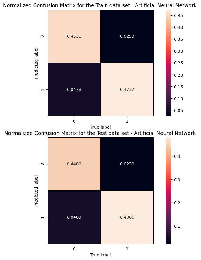
The information from the evaluation metrics can be summarised in a so-called confusion matrix whose elements, from the top-left side, represent TN, FP, FN and TP rates.

print('Cut/Threshold on the ANN output : %.4f \n' % cut_dnn )
print('Confusion matrix ANN\n')

plt.style.use('default') # It's ugly otherwise
plt.figure(figsize=(10,10) )


plt.subplot(2,1,1)
mat_train = confusion_matrix(y_true_train, y_pred_train,sample_weight=w_train,normalize='all')
sns.heatmap(mat_train.T, square=True, annot=True, fmt='.4f', cbar=True,linewidths=1,linecolor='black' )
plt.xlabel('True label')
plt.ylabel('Predicted label');
plt.title('Normalized Confusion Matrix for the Train data set - Artificial Neural Network ')

plt.subplot(2, 1, 2)
mat_test = confusion_matrix(y_true, y_pred ,sample_weight=w_test,normalize='all' )
sns.heatmap(mat_test.T, square=True, annot=True, fmt='.4f', cbar=True,linewidths=1,linecolor='black')
plt.xlabel('True label')
plt.ylabel('Predicted label');
plt.title('Normalized Confusion Matrix for the Test data set - Artificial Neural Network ')

Cut/Threshold on the ANN output : 0.6000 

Confusion matrix ANN

Image Added

An alternative way to check overfitting, and choosing correctly a threshold for selecting signal events, is plotting signal and background ANN predictions for the training and test datasets. If the distributions are quite similar it means that the algorithm learned how to generalize!
For measuring quantitatively the overfitting one can perform a Kolmogorov-Smirnov test that we will not implement here.

References

Attachments