...
Test dataset shape:
(22997, 27)
Test dataset signal shape:
(2870, 5)
Test dataset background shape:
(20127, 5)
Training dataset shape
(91987, 27)
Training signal dataset shape
(11390, 5)
Training background dataset shape
(80597, 5)
df_test.head()
| f_run | f_event | f_weight | f_massjj | f_deltajj | f_mass4l | f_Z1mass | f_Z2mass | f_lept1_pt | f_lept1_eta | f_lept1_phi | f_lept2_pt | f_lept2_eta | f_lept2_phi | f_lept3_pt | f_lept3_eta | f_lept3_phi | f_lept4_pt | f_lept4_eta | f_lept4_phi | f_jet1_pt | f_jet1_eta | f_jet1_phi | f_jet2_pt | f_jet2_eta | f_jet2_phi | isSignal | |
|---|---|---|---|---|---|---|---|---|---|---|---|---|---|---|---|---|---|---|---|---|---|---|---|---|---|---|---|
| 9101 | 1 | 80913 | 0.000075 | 499.415680 | 3.541091 | 123.750252 | 69.386528 | 22.196232 | 47.066288 | -1.938778 | -0.157178 | 24.794939 | -1.477099 | 2.680755 | 21.430199 | -1.085863 | -0.474563 | 16.923937 | 0.011259 | -0.304338 | 83.238281 | -2.022697 | 1.945629 | 84.314346 | 1.518393 | -2.281762 | 1.0 |
| 61307 | 1 | 1799470 | 0.000004 | 1034.700684 | 5.445127 | 123.126251 | 87.025040 | 30.899391 | 54.302334 | 1.254665 | 0.491101 | 34.218605 | 1.576207 | -2.819679 | 24.933231 | 1.195293 | 2.530720 | 11.106866 | 0.836214 | 0.240992 | 88.764404 | -1.835088 | -2.809269 | 52.351109 | 3.610039 | -2.063801 | 0.0 |
| 434065 | 1 | 48636330 | 0.000015 | 131.100220 | 1.032331 | 224.591537 | 90.623093 | 115.573257 | 64.985748 | 1.022329 | 0.020787 | 49.217106 | -0.768105 | 0.152171 | 43.280205 | 0.537557 | -0.211530 | 41.790005 | -0.187201 | 2.840212 | 114.500084 | 0.614150 | 3.130475 | 32.397049 | 1.646480 | -0.925176 | 0.0 |
| 755935 | 1 | 54379498 | 0.000004 | 83.658073 | 1.574079 | 201.779816 | 95.846970 | 85.438805 | 72.073616 | 0.108228 | -2.730205 | 54.219593 | 0.489068 | -1.299269 | 24.958881 | -1.389947 | -2.604218 | 13.022590 | 1.919428 | 1.664050 | 46.515545 | 1.133949 | 0.139815 | 44.397335 | -0.440129 | 0.533251 | 0.0 |
| 504179 | 1 | 98493569 | 0.000001 | 652.359863 | 3.799881 | 335.023987 | 90.216057 | 92.984535 | 126.748039 | 1.168150 | -0.711313 | 87.271675 | -0.707292 |
df_all.head()
| f_run | f_event | f_weight | f_massjj | f_deltajj | f_mass4l | f_Z1mass | f_Z2mass | f_lept1_pt | f_lept1_eta | f_lept1_phi | f_lept2_pt | f_lept2_eta | f_lept2_phi | f_lept3_pt | f_lept3_eta | f_lept3_phi | f_lept4_pt | f_lept4_eta | f_lept4_phi | f_jet1_pt | f_jet1_eta | f_jet1_phi | f_jet2_pt | f_jet2_eta | f_jet2_phi | isSignal | |
|---|---|---|---|---|---|---|---|---|---|---|---|---|---|---|---|---|---|---|---|---|---|---|---|---|---|---|---|
| 9101 | 1 | 80913 | 0.000075 | 499.415680 | 3.541091 | 123.750252 | 69.386528 | 22.196232 | 47.066288 | -1.938778 | -0.157178 | 24.794939 | -1.477099 | 2.680755 | 21.430199 | -1.085863 | -0.474563 | 16.923937 | 0.011259 | -0.304338 | 83.238281 | -2.022697 | 1.945629 | 84.314346 | 1.518393 | -2.281762 | 1.0 |
| 61307 | 1 | 1799470 | 0.000004 | 1034.700684 | 5.445127 | 123.126251 | 87.025040 | 30.899391 | 54.302334 | 1.254665 | 0.491101 | 34.218605 | 1.576207 | -2.819679 | 24.933231 | 1.195293 | 2.530720 | 11.106866 | 0.836214 | 0.240992 | 88.764404 | -1.835088 | -2.809269 | 52.351109 | 3.610039 | -2.063801 | 0.0 |
| 434065 | 1 | 48636330 | 0.000015 | 131.100220 | 1.032331 | 224.591537 | 90.623093 | 115.573257 | 64.985748 | 1.022329 | 0.020787 | 49.217106 | -0.768105 | 0.152171 | 43.280205 | 0.537557 | -0.211530 | 41.790005 | -0.187201 | 2.840212 | 114.500084 | 0.614150 | 3.130475 | 32.397049 | 1.646480 | -0.925176 | 0.0 |
| 755935 | 1 | 54379498 | 0.000004 | 83.658073 | 1.574079 | 201.779816 | 95.846970 | 85.438805 | 72.073616 | 0.108228 | -2.730205 | 54.219593 | 0.489068 | -1.299269 | 24.958881 | -1.389947 | -2.604218 | 13.022590 | 1.919428 | 1.664050 | 46.515545 | 1.133949 | 0.139815 | 44.397335 | -0.440129 | 0.533251 | 0.0 |
| 504179 | 1 | 98493569 | 0.000001 | 652.359863 | 3.799881 | 335.023987 | 90.216057 | 92.984535 | 126.748039 | 1.168150 | -0.711313 | 87.271675 | -0.707292 | 1.167732 | 41.464527 | -0.289785 | -0.509481 | 14.898630 | -0.470465 | 0.317107 | 99.428864 | -3.475805 | 2.928077 | 99.210449 | 0.324076 | -3.102045 | 0.0 |
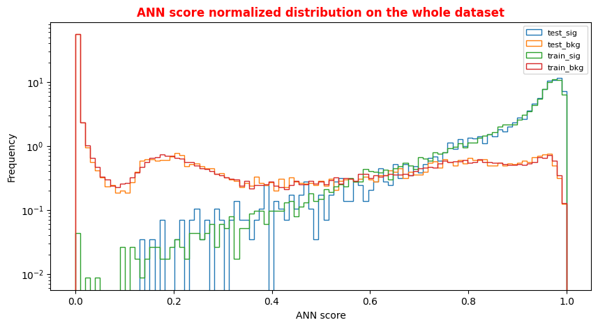
# Normalized Distribution of the ANN score for the whole dataset
# ax = plt.subplot(4, 2, 4)
X = np.linspace(0.0, 1.0, 100) #100 numbers between 0 and 1
plt.rcParams['figure.figsize'] = (10,5)
hist_test_sig = plt.hist(Y_test_sig, bins=X, label='test_sig',histtype='step',log=True,density=1)
hist_test_bkg = plt.hist(Y_test_bkg, bins=X, label='test_bkg',histtype='step',log=True,density=1)
hist_train_sig = plt.hist(Y_train_sig, bins=X, label='train_sig',histtype='step',log=True,density=1)
hist_train_bkg = plt.hist(Y_train_bkg, bins=X, label='train_bkg',histtype='step',log=True,density=1)
plt.xlabel('ANN score')
plt.ylabel('Frequency')
plt.legend( loc='upper right',prop={'size': 8} )
plt.title('ANN score normalized distribution on the whole dataset',fontsize=12,fontweight='bold', color='r')
plt.show()
Exercise 1 - Random Forest performance
Evaluate the performance of the Random Forest algorithm. Hint: use the predict_proba method this time!
In [ ]:
# Get RF model predictions and performance metric curves, after having trained the model
# Get RF model predictions and performance metric curves, after having trained the model

# Do it for the test dataset:
y_pred_rfc=randomforest.predict(X_test[:,0:NINPUT])
y_pred_rfc_prob= randomforest.predict_proba(X_test[:,0:NINPUT])
y_pred_rfc_proba = y_pred_rfc_prob[:,-1]
p_rf,r_rf,t_rf= precision_recall_curve(Y_test, probas_pred=y_pred_rfc_proba , sample_weight=w_test)
fpr_rf, tpr_rf, thresholds_rf = roc_curve(Y_test, y_score=y_pred_rfc_proba, sample_weight=w_test  )

# Do the same for the training dataset:
y_pred_rfc_train=randomforest.predict(X_train_val[:,0:NINPUT])
y_pred_rfc_train_prob= randomforest.predict_proba(X_train_val[:,0:NINPUT])
y_pred_rfc_train_proba = y_pred_rfc_train_prob[:,-1] #last element associated to the signal probability
p_train_rf, r_train_rf, t_train_rf = precision_recall_curve(Y_train_val, y_pred_rfc_train_proba, sample_weight=w_train)
fpr_train_rf, tpr_train_rf, thresholds_train_rf = roc_curve(Y_train_val, y_pred_rfc_train_proba, sample_weight=w_train)
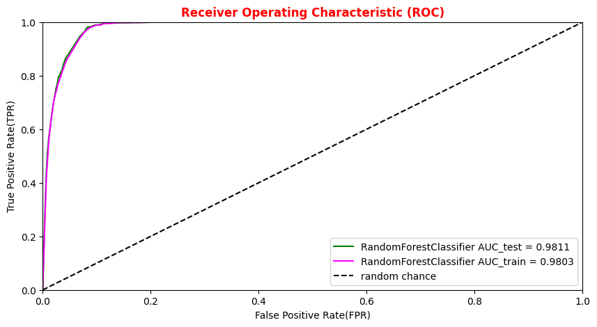
# Plotting the ROC curve for the Random Forest algorithm
roc_auc_rf = auc(fpr_rf,tpr_rf)
roc_auc_rf_train = auc(fpr_train_rf,tpr_train_rf)

plt.rcParams['figure.figsize'] = (10,5)
#Random Forest 1st method
plt.plot(fpr_rf,tpr_rf,  color='green', label='RandomForestClassifier AUC_test = %.4f' % (roc_auc_rf))
plt.plot(fpr_train_rf,tpr_train_rf, color='magenta', label='RandomForestClassifier AUC_train = %.4f' % (roc_auc_rf_train))
#Random Forest 2nd method : use the sklearn function "plot_roc_curve"
#rfc_disp = plot_roc_curve(rfc, X_train_val,Y_train_val,color='brown',ax=ax, sample_weight=w_train )
#rfc_disp = plot_roc_curve(rfc, X_test, Y_test, color='grey',ax=ax, sample_weight=w_test)
#random chance
plt.plot([0, 1], [0, 1], linestyle='--', color='k', label='random chance')
plt.xlim([0, 1.0]) #fpr
plt.ylim([0, 1.0]) #tpr
plt.xlabel('False Positive Rate(FPR)')
plt.ylabel('True Positive Rate(TPR)')
plt.title('Receiver Operating Characteristic (ROC)',fontsize=12,fontweight='bold', color='r')
plt.legend(loc="lower right")
plt.show()
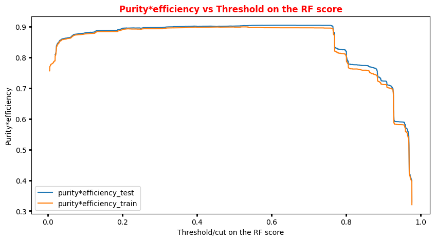
# Plot Efficiency x Purity -- Random Forest

# Other metrics:
# plt.plot(t_rf, p_rf[:-1], label='purity_test')
# plt.plot(t_train_rf, p_train_rf[:-1], label='purity_test')
# plt.plot(t_rf, r_rf[:-1], label='efficiency_test')
# plt.plot(t_train_rf, r_train_rf[:-1], label='efficiency_train')
plt.rcParams['figure.figsize'] = (10,5)
plt.plot(t_rf,p_rf[:-1]*r_rf[:-1],label='purity*efficiency_test')
plt.plot(t_train_rf,p_train_rf[:-1]*r_train_rf[:-1],label='purity*efficiency_train')
plt.ylabel('Purity*efficiency')
plt.xlabel('Threshold/cut on the RF score')
plt.title('Purity*efficiency vs Threshold on the RF score',fontsize=12,fontweight='bold', color='r')
plt.tick_params(width=2, grid_alpha=0.5)
plt.legend(markerscale=50)
plt.show()
# Random Forest score for training and test datasets (bkg and sig)

Y_sig_rfc = randomforest.predict_proba(X_sig) #probability of belonging to the signal(bkg) class for all signal events
Y_bkg_rfc = randomforest.predict_proba(X_bkg)  #probability of belonging to the signal(bkg) class for all bkg events
Y_test_sig_rf= randomforest.predict_proba(X_test_sig) # the same for all signal events in the test dataset
Y_test_bkg_rf = randomforest.predict_proba(X_test_bkg) # the same for all bkg events in the test dataset
Y_train_sig_rf = randomforest.predict_proba(X_train_sig) # the same for all sig events in the training dataset
Y_train_bkg_rf = randomforest.predict_proba(X_train_bkg) # the same for all bkg events in the training dataset
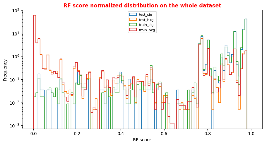
# Random Forest score Plot for the whole dataset
X = np.linspace(0.0, 1.0, 100) #100 numbers between 0 and 1
plt.rcParams['figure.figsize'] = (10,5)
hist_test_sig = plt.hist(Y_test_sig_rf[:,1], bins=X, label='test_sig',histtype='step',log=True,density=1 )
hist_test_bkg = plt.hist(Y_test_bkg_rf[:,1], bins=X, label='test_bkg',histtype='step',log=True,density=1)
hist_train_sig = plt.hist(Y_train_sig_rf[:,1], bins=X, label='train_sig',histtype='step',log=True,density=1)
hist_train_bkg = plt.hist(Y_train_bkg_rf[:,1], bins=X, label='train_bkg',histtype='step',log=True,density=1)
plt.xlabel('RF score')
plt.ylabel('Frequency')
plt.legend( loc='upper center',prop={'size': 8} )
plt.title('RF score normalized distribution on the whole dataset',fontsize=12,fontweight='bold', color='r')
plt.show()
# We choose a threshold on the RF score for labelling signal and background events looking at the
# previous plots
cut_rf=0.6

y_pred_rfc[y_pred_rfc >= cut_rf]=1 #classify them as signal
y_pred_rfc[y_pred_rfc < cut_rf]=0 #classify them as background

#print("y_pred_rfc.shape",y_pred_rfc.shape)
#print("y_pred_rfc",y_pred_rfc)

#Metrics for the RandomForest
accuracy_rfc  = accuracy_score(y_true, y_pred_rfc, sample_weight=w_test) #fraction of correctly classified events
precision_rfc = precision_score(y_true, y_pred_rfc, sample_weight=w_test) #Precision of the positive class in binary classification
recall_rfc    = recall_score(y_true, y_pred_rfc, sample_weight=w_test) #Recall of the positive class in binary classification
f1_rfc = 2*precision_rfc*recall_rfc/(precision_rfc+recall_rfc)
print('Cut/Threshold on the Random Forest output : %.4f' % cut_rf)
print('Random Forest Test Accuracy: %.4f' % accuracy_rfc)
print('Random Forest Test Precision/Purity:  %.4f' % precision_rfc)
print('Random Forest Test Sensitivity/Recall/TPR/Signal Efficiency: %.4f' % recall_rfc)
print('RF Test F1:   %.4f' %f1_rfc)
print('')
Cut/Threshold on the Random Forest output : 0.6000
Random Forest Test Accuracy: 0.9471
Random Forest Test Precision/Purity:  0.9180
Random Forest Test Sensitivity/Recall/TPR/Signal Efficiency: 0.9827
RF Test F1: 0.9492print('Cut/Threshold on the Random Forest output : %.4f' % cut_rf) #cm_rfc = confusion_matrix( y_true, y_pred_rfc, sample_weight=w_test) #disp_rfc = ConfusionMatrixDisplay(confusion_matrix=cm_rfc, display_labels='bs' ) #disp_rfc.plot() plt.style.use('default') # It's ugly otherwise plt.figure(figsize=(10,10) ) plt.subplot(2,1,1) mat = confusion_matrix(y_true_train, y_pred_rfc_train,sample_weight=w_train,normalize='all' ) sns.heatmap(mat.T, square=True, annot=True, fmt='.4f', cbar=True,linewidths=1,linecolor='black') plt.xlabel('True label') plt.ylabel('Predicted label'); plt.title('Normalized Confusion Matrix for the Train data set - Random Forest ' ) plt.subplot(2, 1, 2) mat = confusion_matrix(y_true, y_pred_rfc ,sample_weight=w_test, normalize='all' ) sns.heatmap(mat.T, square=True, annot=True, fmt='.4f' , cbar=True,linewidths=1,linecolor='black') plt.xlabel('True label') plt.ylabel('Predicted label'); plt.title('Normalized Confusion Matrix for the Test data set - Random Forest ')
Cut/Threshold on the Random Forest output : 0.6000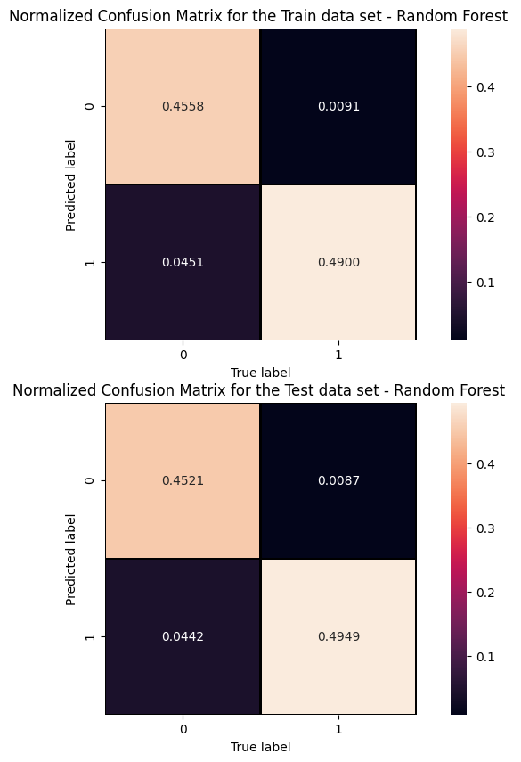
##Superimposition RF and ANN ROC curves
plt.rcParams['figure.figsize'] = (10,5)
plt.plot(fpr_train, tpr_train, color='red', label='NN AUC_train = %.4f' % (roc_auc_train))
plt.plot(fpr, tpr,  color='cyan', label='NN AUC_test = %.4f' % (roc_auc))
#Random Forest 1st method
plt.plot(fpr_train_rf,tpr_train_rf, color='blue', label='RandomForestClassifier AUC_train = %.4f' % (roc_auc_rf_train))
plt.plot(fpr_rf,tpr_rf, color='grey', label='RandomForestClassifier AUC_test = %.4f' % (roc_auc_rf))
#Random Forest 2nd method
#rfc_disp = plot_roc_curve(rfc, X_train_val,Y_train_val,color='brown',ax=ax, sample_weight=w_train )
#rfc_disp = plot_roc_curve(rfc, X_test, Y_test, color='grey',ax=ax, sample_weight=w_test)
#random chance
plt.plot([0, 1], [0, 1], linestyle='--', color='k', label='random chance')
plt.xlim([0, 1.0]) #fpr
plt.ylim([0, 1.0]) #tpr
plt.title('Receiver Operating Characteristic (ROC)',fontsize=12,fontweight='bold', color='r')
plt.xlabel('False Positive Rate(FPR)')
plt.ylabel('True Positive Rate(TPR)')
plt.legend(loc="lower right")
plt.show()