...
Moreover, you will look at the physical observables that you can use to train the ML algorithms.In [ ]:
#import#import scientific libraries

import uproot
import numpy as np
import pandas as pd
import h5py
import seaborn as sns

from sklearn.utils import shuffle
from sklearn.model_selection import train_test_split
from sklearn.datasets import make_classification

import tensorflow as tf
from tensorflow import keras
from tensorflow.keras.models import Sequential, Model
from tensorflow.keras.optimizers import SGD, Adam, RMSprop, Adagrad, Adadelta
from tensorflow.keras.layers import Input, Activation, Dense, Dropout
from tensorflow.keras.callbacks import EarlyStopping, ReduceLROnPlateau, ModelCheckpoint
from tensorflow.keras import utils
from tensorflow import random as tf_random
from keras.utils import plot_model
import random as python_random
# Fix random seed for reproducibility

# The below is necessary for starting Numpy generated random numbers
# in a well-defined initial state.
seed = 7
np.random.seed(seed)

# The below is necessary for starting core Python generated random numbers
# in a well-defined state.
python_random.seed(seed)

# The below set_seed() will make random number generation
# in the TensorFlow backend have a well-defined initial state.
# For further details, see: https://www.tensorflow.org/api_docs/python/tf/random/set_seed
tf_random.set_seed(seed)

treename = 'HZZ4LeptonsAnalysisReduced'
filename = {}
upfile = {}
params = {}
df = {}

# Define what are the ROOT files we are interested in (for the two categories,
# signal and background)

filename['sig'] = 'VBF_HToZZTo4mu.root'
filename['bkg_ggHtoZZto4mu'] = 'GluGluHToZZTo4mu.root'
filename['bkg_ZZto4mu'] = 'ZZTo4mu.root'
#filename['bkg_ttH_HToZZ_4mu.root']= 'ttH_HToZZ_4mu.root'
#filename['sig'] = 'VBF_HToZZTo4e.root'
#filename['bkg_ggHtoZZto4e'] = 'GluGluHToZZTo4e.root'
#filename['bkg_ZZto4e'] = 'ZZTo4e.root'

# Variables from Root Tree that must be copyed to PANDA dataframe (df)
VARS = [ 'f_run', 'f_event', 'f_weight', \
        'f_massjj', 'f_deltajj', 'f_mass4l', 'f_Z1mass' , 'f_Z2mass', \
        'f_lept1_pt','f_lept1_eta','f_lept1_phi', \
        'f_lept2_pt','f_lept2_eta','f_lept2_phi', \
        'f_lept3_pt','f_lept3_eta','f_lept3_phi', \
        'f_lept4_pt','f_lept4_eta','f_lept4_phi', \
        'f_jet1_pt','f_jet1_eta','f_jet1_phi', \
        'f_jet2_pt','f_jet2_eta','f_jet2_phi' ]

#checking the dimensions of the df , 26 variables
NDIM = len(VARS)

print("Number of kinematic variables imported from the ROOT files = %d"% NDIM)

upfile['sig'] = uproot.open(filename['sig'])
upfile['bkg_ggHtoZZto4mu'] = uproot.open(filename['bkg_ggHtoZZto4mu'])
upfile['bkg_ZZto4mu'] = uproot.open(filename['bkg_ZZto4mu'])
#upfile['bkg_ttH_HToZZ_4mu.root'] = uproot.open(filename['bkg_ttH_HToZZ_4mu'])
Number of kinematic variables imported from the ROOT files = 26
Let's see what you have uploaded in your Colab notebook!
# Look at the signal and bkg events before applying physical requirement

df#upfile['sig'] = uprootpd.openDataFrame(filenameupfile['sig'])]
#upfile['bkg_ggHtoZZto4e'] = uproot.open(filename['bkg_ggHtoZZto4e'])
#upfile['bkg_ZZto4e'] = uproot.open(filename['bkg_ZZto4e'])
Number of kinematic variables imported from the ROOT files = 26
Let's see what you have uploaded in your Colab notebook!
# Look at the signal and bkg events before applying physical requirement

df['sig'] = pd.DataFrame(upfile['sig'][treename].[treename].arrays(VARS, library="np"),columns=VARS)
print(df['sig'].shape)
...
The first 2 columns contain information that is provided by experiments at the LHC that will not be used in the training of our Machine Learning algorithms, therefore we skip our explanation to the next columns.
The next variable is the
f_weights. This corresponds to the probability of having that particular kind of physical process on the whole experiment. Indeed, it is a product of Branching Ratio (BR), geometrical acceptance of the detector, and kinematic phase-space. It is very important for the training phase and you will use it later.The variables
f_massjj,f_deltajj,f_mass4l,f_Z1mass, andf_Z2massare named high-level features (event features) since they contain overall information about the final-state particles (the mass of the two jets, their separation in space, the invariant mass of the four leptons, the masses of the two Z bosons). Note that themass is lighter w.r.t. the
one. Why is that? In the Higgs boson production (hypothesis of mass = 125 GeV) only one of the Z bosons is an actual particle that has the nominal mass of 91.18 GeV. The other one is a virtual (off-mass shell) particle.
The remnant columns represent the low-level features (object kinematics observables), the basic measurements which are made by the detectors for the individual final state objects (in our case four charged leptons and jets) such as
f_lept1(2,3,4)_pt(phi,eta)corresponding to their transverse momentum and the spatial distribution of their tracks ().
The same comments hold for the background datasets:
objects (in our case four charged leptons and jets) such as
f_lept1(2,3,4)_pt(phi,eta)corresponding to their transverse momentum and the spatial distribution of their tracks (
The same comments hold for the background datasets:
df['bkg_ggHtoZZto4mu# Part of the code in "#" can be used in the second part of the exercise
# for trying to use alternative datasets for the training of our ML algorithms

#df['bkg'] = pd.DataFrame(upfile['bkg'][treename].arrays(VARS, library="np"),columns=VARS)
#df['bkg'].head()
df['bkg_ggHtoZZto4mu'] = pd.DataFrame(upfile['bkg_ggHtoZZto4mu'][treename].arrays(VARS, library="np"),columns=VARS)
df['bkg_ggHtoZZto4mu'].head()
#df['bkg_ggHtoZZto4e'] = pd.DataFrame(upfile['bkg_ggHtoZZto4e'][treename].arrays(VARS, library="np"),columns=VARS)
#df['bkg_ggHtoZZto4e'].head()
#df['bkg_ZZto4e'] = pd.DataFrame(upfile['bkg_ZZto4eggHtoZZto4mu'][treename].arrays(VARS, library="np"),columns=VARS)
#dfdf['bkg_ZZto4eggHtoZZto4mu'].head()
Out[ ]:
| f_run | f_event | f_weight | f_massjj | f_deltajj | f_mass4l | f_Z1mass | f_Z2mass | f_lept1_pt | f_lept1_eta | f_lept1_phi | f_lept2_pt | f_lept2_eta | f_lept2_phi | f_lept3_pt | f_lept3_eta | f_lept3_phi | f_lept4_pt | f_lept4_eta | f_lept4_phi | f_jet1_pt | f_jet1_eta | f_jet1_phi | f_jet2_pt | f_jet2_eta | f_jet2_phi | |
|---|---|---|---|---|---|---|---|---|---|---|---|---|---|---|---|---|---|---|---|---|---|---|---|---|---|---|
| 0 | 1 | 581632 | 0.000225 | -999.0 | -999.0 | 120.101105 | 88.262352 | 22.051540 | 57.572330 | -0.433627 | -0.886073 | 56.933735 | 0.496556 | 0.404675 | 33.584896 | -0.037387 | 0.291866 | 10.881461 | -1.112960 | 0.051097 | 73.541260 | 1.683280 | 2.736636 | -999.0 | -999.0 | -999.0 |
| 1 | 1 | 581659 | 0.000277 | -999.0 | -999.0 | 124.592812 | 82.174683 | 17.613417 | 50.365120 | 0.001362 | 0.933713 | 31.548225 | 0.598417 | -1.863556 | 22.758055 | 0.220867 | -2.767246 | 17.264626 | 0.361964 | -1.859138 | -999.000000 | -999.000000 | -999.000000 | -999.0 | -999.0 | -999.0 |
| 2 | 1 | 581671 | 0.000278 | -999.0 | -999.0 | 125.692230 | 79.915764 | 29.998011 | 72.355927 | -0.238323 | -2.335623 | 20.644920 | -0.241560 | 1.855536 | 16.031651 | -1.446993 | 1.185016 | 11.068296 | 0.366903 | -0.606845 | 64.440544 | 1.886244 | 1.635723 | -999.0 | -999.0 | -999.0 |
| 3 | 1 | 581724 | 0.000336 | -999.0 | -999.0 | 125.027504 | 85.200958 | 23.440151 | 43.059235 | 0.759979 | -1.714778 | 19.248983 | 0.535979 | 0.420337 | 16.595169 | -1.330326 | 1.656061 | 11.407483 | -0.686118 | 1.295116 | -999.000000 | -999.000000 | -999.000000 | -999.0 | -999.0 | -999.0 |
| 4 | 1 | 581744 | 0.000273 | -999.0 | -999.0 | 124.917282 | 65.971390 | 14.968305 | 52.585011 | -0.656421 | -2.933651 | 35.095982 | -1.002568 | 0.865173 | 28.146715 | -0.730926 | -0.876442 | 8.034222 | -1.094436 | 1.783626 | -999.000000 |
...
# Let's merge our background processes together!
df['bkg'] = pd.concat([df['bkg_ZZto4mu'],df['bkg_ggHtoZZto4mu']])
# Let's shuffle them!
df['bkg']= shuffle(df['bkg'])
# Let's see its shape!
print(df['bkg'].shape)
#print(len(df['bkg']))
#print(len(df['bkg_ZZto4mu']))
#print(len(df['bkg_ggHtoZZto4mu']))
#print(len(df['bkg_ggHtoZZto4e']))
#print(len(df['bkg_ZZto4e']))
(952342, 26)
Note that the background datasets seem to have a very large number of events! Is that true? Do all physical variables have meaningful values? Let's make physical selection requirements!
...
Cut/Threshold on the ANN output : 0.6000 Confusion matrix ANN
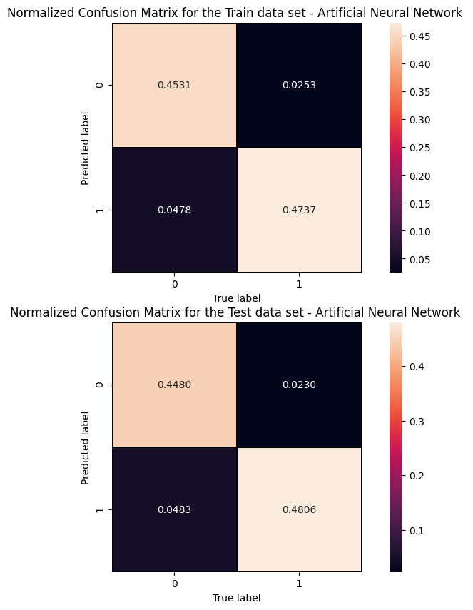
An alternative way to check overfitting, and choosing correctly a threshold for selecting signal events, is plotting signal and background ANN predictions for the training and test datasets. If the distributions are quite similar it means that the algorithm learned how to generalize!
For measuring quantitatively the overfitting one can perform a Kolmogorov-Smirnov test that we will not implement here.
...
# Get RF model predictions and performance metric curves, after having trained the model
# Get RF model predictions and performance metric curves, after having trained the model

# Do it for the test dataset:
y_pred_rfc=randomforest.predict(X_test[:,0:NINPUT])
y_pred_rfc_prob= randomforest.predict_proba(X_test[:,0:NINPUT])
y_pred_rfc_proba = y_pred_rfc_prob[:,-1]
p_rf,r_rf,t_rf= precision_recall_curve(Y_test, probas_pred=y_pred_rfc_proba , sample_weight=w_test)
fpr_rf, tpr_rf, thresholds_rf = roc_curve(Y_test, y_score=y_pred_rfc_proba, sample_weight=w_test  )

# Do the same for the training dataset:
y_pred_rfc_train=randomforest.predict(X_train_val[:,0:NINPUT])
y_pred_rfc_train_prob= randomforest.predict_proba(X_train_val[:,0:NINPUT])
y_pred_rfc_train_proba = y_pred_rfc_train_prob[:,-1] #last element associated to the signal probability
p_train_rf, r_train_rf, t_train_rf = precision_recall_curve(Y_train_val, y_pred_rfc_train_proba, sample_weight=w_train)
fpr_train_rf, tpr_train_rf, thresholds_train_rf = roc_curve(Y_train_val, y_pred_rfc_train_proba, sample_weight=w_train)
...
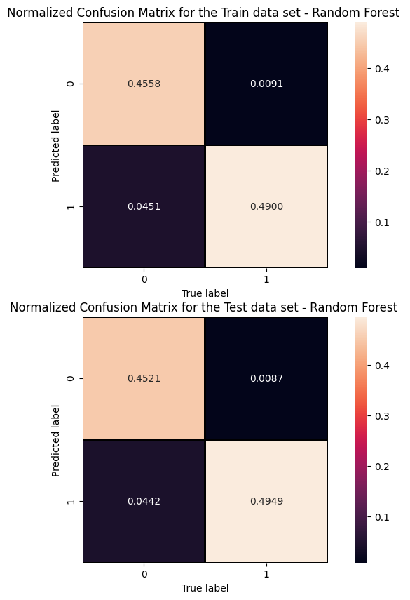
Cut/Threshold on the Random Forest output : 0.6000
##Superimposition RF and ANN ROC curves
plt.rcParams['figure.figsize'] = (10,5)
plt.plot(fpr_train, tpr_train, color='red', label='NN AUC_train = %.4f' % (roc_auc_train))
plt.plot(fpr, tpr,  color='cyan', label='NN AUC_test = %.4f' % (roc_auc))
#Random Forest 1st method
plt.plot(fpr_train_rf,tpr_train_rf, color='blue', label='RandomForestClassifier AUC_train = %.4f' % (roc_auc_rf_train))
plt.plot(fpr_rf,tpr_rf, color='grey', label='RandomForestClassifier AUC_test = %.4f' % (roc_auc_rf))
#Random Forest 2nd method
#rfc_disp = plot_roc_curve(rfc, X_train_val,Y_train_val,color='brown',ax=ax, sample_weight=w_train )
#rfc_disp = plot_roc_curve(rfc, X_test, Y_test, color='grey',ax=ax, sample_weight=w_test)
#random chance
plt.plot([0, 1], [0, 1], linestyle='--', color='k', label='random chance')
plt.xlim([0, 1.0]) #fpr
plt.ylim([0, 1.0]) #tpr
plt.title('Receiver Operating Characteristic (ROC)',fontsize=12,fontweight='bold', color='r')
plt.xlabel('False Positive Rate(FPR)')
plt.ylabel('True Positive Rate(TPR)')
plt.legend(loc="lower right")
plt.show()
...