| Table of Contents |
|---|
Author(s)
| Name | Institution | Mail Address | Social Contacts |
|---|---|---|---|
| Brunella D'Anzi | INFN Sezione di Bari | brunella.d'anzi@cern.ch | Skype: live:ary.d.anzi_1; Linkedin: brunella-d-anzi |
| Nicola De Filippis | INFN Sezione di Bari | nicola.defilippis@ba.infn.it | |
Domenico Diacono | INFN Sezione di Bari | domenico.diacono@ba.infn.it | |
| Walaa Elmetenawee | INFN Sezione di Bari | walaa.elmetenawee@cern.ch | |
| Giorgia Miniello | INFN Sezione di Bari | giorgia.miniello@ba.infn.it | |
| Andre Sznajder | Rio de Janeiro State University | sznajder.andre@gmail.com |
How to Obtain Support
| brunella.d'anzi@cern.ch,giorgia.miniello@ba.infn.it | |
| Social | Skype: live:ary.d.anzi_1; Linkedin: brunella-d-anzi |
General Information
| ML/DL Technologies | Artificial Neural Networks (ANNs), Random Forests (RFs) |
|---|---|
| Science Fields | High Energy Physics |
| Difficulty | Low |
| Language | English |
| Type | fully annotated and runnable |
Software and Tools
| Programming Language | Python |
|---|---|
| ML Toolset | |
| Additional libraries | uproot, NumPy, pandas,h5py,seaborn,matplotlib |
| Suggested Environments | Google's Colaboratory |
Needed datasets
| Data Creator | CMS Experiment |
|---|---|
| Data Type | Simulation |
| Data Size | 2 GB |
| Data Source | Cloud@ReCaS-Bari |
Short Description of the Use Case
Introduction to the statistical analysis problem
In this exercise, you will perform a binary classification task using Monte Carlo simulated samples representing the Vector Boson Fusion (VBF) Higgs boson production in the four-lepton final state signal and its main background processes at the Large Hadron Collider (LHC) experiments. Two Machine Learning (ML) algorithms will be implemented: an Artificial Neural Network (ANN) and a Random Forest (RF).
- You will learn how a multivariate analysis algorithm works (see the below introduction) and more specifically how a Machine Learning model must be implemented;
- you will acquire basic knowledge about the *Higgs boson physics* as described by the Standard Model. During the exercise you will be invited to plot some physical quantities in order to understand what is the underlying Particle Physics problem;
- you will be invited to *change hyperparameters* of the ANN and the RF parameters to understand better what are the consequences in terms of the models' performances;
- you will understand that the choice of the *input variables* is a key task of a Machine Learning algorithm since an optimal choice allows achieving the best possible performances;
- moreover, you will have the possibility of changing the background datasets, the decay channels of the final state particles, and seeing how the ML algorithms' performance changes.
Multivariate Analysis and Machine Learning algorithms: basic concepts
Multivariate Analysis algorithms receive as input a set of discriminating variables. Each variable alone does not allow to reach an optimal discrimination power between two categories (we will focus on a binary task in this exercise). Therefore the algorithms compute an output that combines the input variables.
...
A description of the Artificial Neural Network and Random Forest algorithms is inserted in the notebook itself.
Particle Physics basic concepts: the Standard Model and the Higgs boson
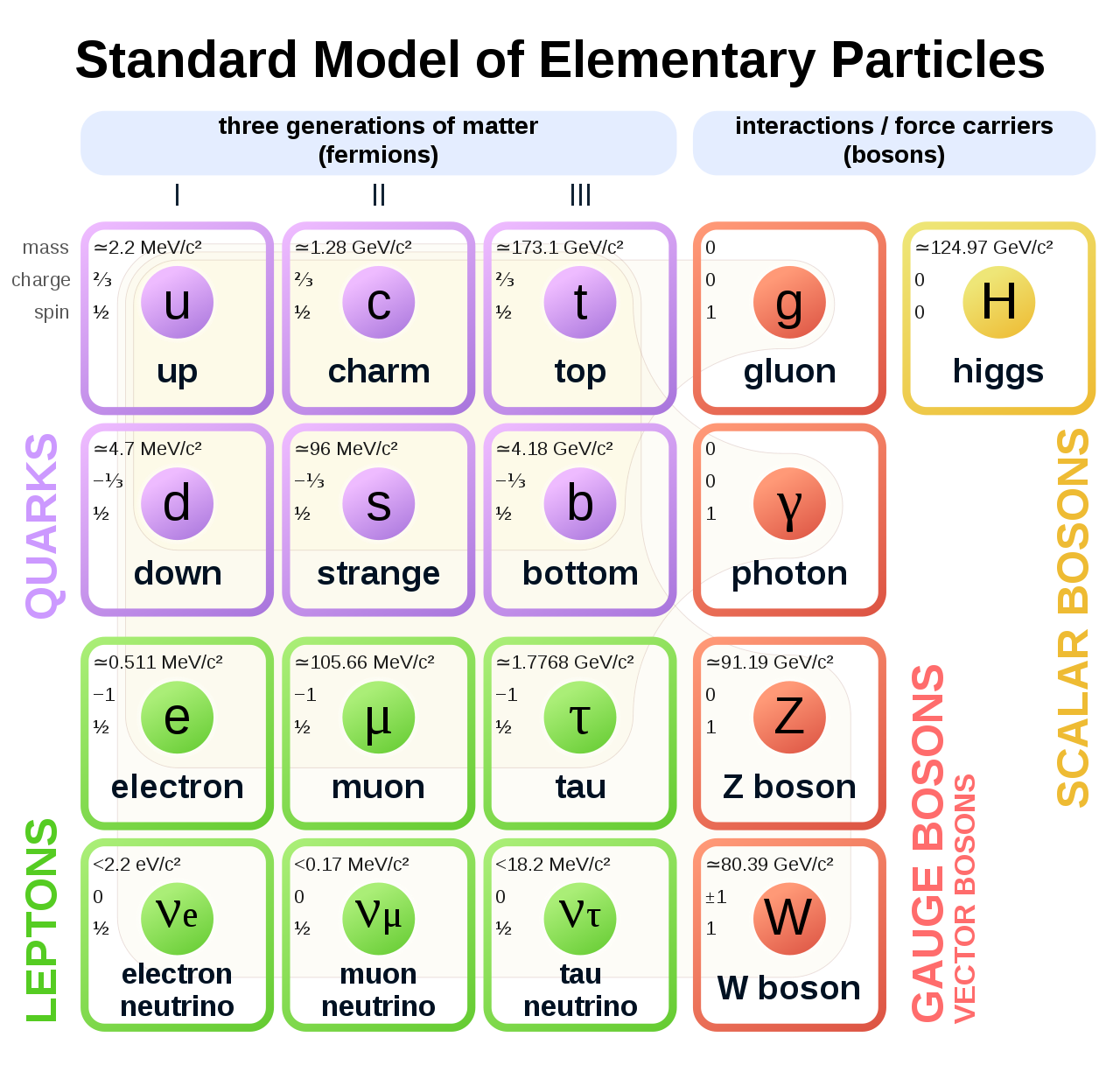
The Standard Model of elementary particles represents our knowledge of the microscopic world. It describes the matter constituents (quarks and leptons) and their interactions (mediated by bosons), which are the electromagnetic, the weak, and the strong interactions.
Among all these particles, the Higgs boson still represents a very peculiar case. It is the second heaviest known elementary particle (mass of 125 GeV) after the top quark (175 GeV).
The ideal tool for measuring the Higgs boson properties is a particle collider. The Large Hadron Collider (LHC), situated nearby Geneva, between France and Switzerland, is the largest proton-proton collider ever built on Earth. It consists of a 27 km circumference ring, where proton beams are smashed at a center-of-mass energy of 13 TeV (99.999999% of the speed of light). At the LHC, 40 Million collisions / second occurs, providing an enormous amount of data. Thanks to these data, ATLAS and CMS experiments discovered the missing piece of the Standard Model, the Higgs boson, in 2012.
During a collision, the energy is so high that protons are "broken" into their fundamental components, i.e. quarks and gluons, that can interact together, producing particles that we don't observe in our everyday life, such as the Higgs boson. The production of a Higgs boson via a vector boson fusion (VBF) mechanism is, by the way, a relatively "rare" phenomenon, since there are other physical processes that occur way more often, such as those initiated by strong interaction, producing the Higgs boson by the so-called gluon-gluon fusion (ggH) production process. In High Energy Physics, we speak about the cross-section of a physics process. We say that the Higgs boson production via the vector boson fusion mechanism has a smaller cross-section than the production of the same boson (scalar particle) via the ggH mechanism.
The experimental consequence is that distinguishing the two processes, which are characterized by the decay products, can be extremely difficult, given that the latter phenomenon has a way larger probability to happen. In the exercise, we will propose to merge different backgrounds to be distinguished from the signal events.
Experimental signature of the Higgs boson in a particle detector
Let's first understand what are the experimental signatures and how the LHC's detectors work. As an example, this is a sketch of the Compact Muon Solenoid (CMS) detector.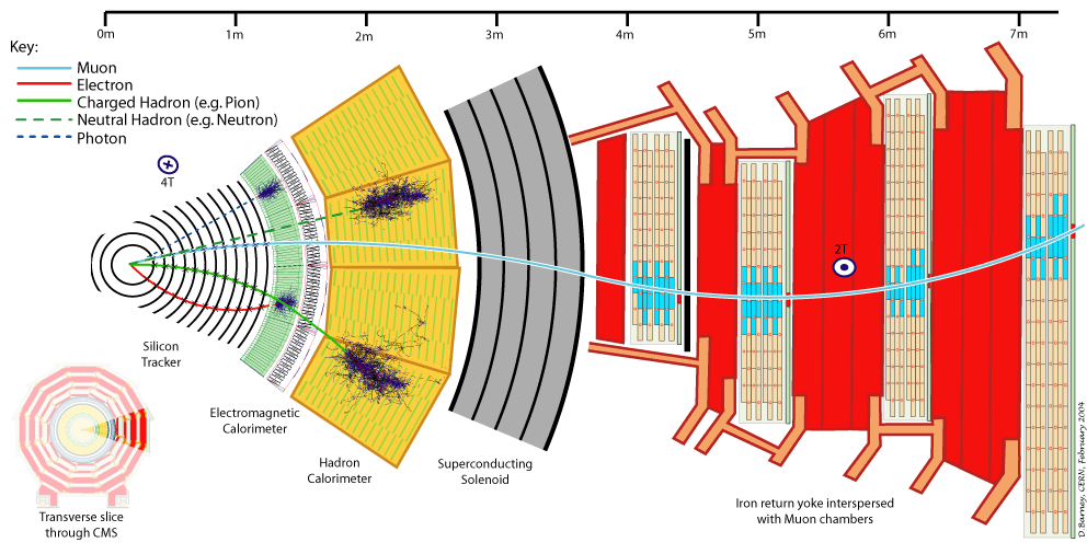
A collider detector is organized in layers: each layer is able to distinguish and measure different particles and their properties. For example, the silicon tracker detects each particle that is charged. The electromagnetic calorimeter detects photons and electrons. The hadronic calorimeter detects hadrons (such as protons and neutrons). The muon chambers detect muons (that have a long lifetime and travel through the inner layers).
...
Our physics problem consists of detecting the so-called golden channel H→ ZZ*→ l+ l- l'+ l'- which is one of the possible Higgs boson's decays: its name is due to the fact that it has the clearest and cleanest signature of all the possible Higgs boson decay modes. The decay chain is sketched here: the Higgs boson decays into Z boson pairs, which in turn decay into a lepton pair (in the picture, muon-antimuon or electron-positron pairs). In this exercise, we will use only datasets concerning the 4mu decay channel and the datasets about the 4e channel are given to you to be analyzed as an optional exercise. At the LHC experiments, the decay channel 2e2mu is also widely analyzed.
Data exploration
In this exercise we are mainly interested in the following ROOT files (you may look at the web page ROOT file if you would like to learn more about which kind of objects you can store in them):
...
We will use some of them for training our Machine Learning algorithms.
How to execute it
Use Googe Colab
What is Google Colab?
Google's Colaboratory is a free online cloud-based Jupyter notebook environment on Google-hosted machines, with some added features, like the possibility to attach a GPU or a TPU if needed with 12 hours of continuous execution time. After that, the whole virtual machine is cleared and one has to start again. The user can run multiple CPU, GPU, and TPU instances simultaneously, but the resources are shared between these instances.
Open the Use Case Colab Notebook
The notebook for this tutorial can be found here. The .ipynb file is available in the attachment section and in this GitHub repository.
...
In order to do this, you must have a personal Google account.
Input files
The datasets files are stored on Recas Bari's ownCloud and are automatically loaded by the notebook. In case, they are also available here (4 muons decay channel) for the main exercise and here (4 electrons decay channel) for the optional exercise.
In the following, the most important excerpts are described.
Annotated Description
Load data using PANDAS data frames
Now you can start using your data and load three different NumPy arrays! One corresponds to the VBF signal and the other two will represent the Higgs boson production via the strong interaction processes (in jargon, QCD)
and
that will be used as a merged background.
...
# Concatenate the signal and background dfs in a single data frame
df_all = pd.concat([df['sig'],df['bkg']])

# Random shuffles the data set to mix signal and background events
# before the splitting between train and test datasets
df_all = shuffle(df_all)
Preparing input features for the ML algorithms
We have our data set ready to train our ML algorithms! Before doing that we have to decide from which input variables the computer algorithms have to learn to distinguish between signal and background events.
...
Number NN input variables= 5
NN input variables= ['f_massjj', 'f_deltajj', 'f_mass4l', 'f_Z1mass', 'f_Z2mass']
(114984, 5)
(114984, 1)
(114984, 1)
Dividing the data into testing and training data set
You can split now the datasets into two parts (one for the training and validation steps and one for testing phase).
...
X (features) before splitting
(114984, 5)
X (features) splitting between test and training
Test:
(22997, 5)
Training:
(91987, 5)
Y (target) before splitting
(114984, 1)
Y (target) splitting between test and training
Test:
(22997, 1)
Training:
(91987, 1)
W (weights) before splitting
(114984, 1)
W (weights) splitting between test and training
Test:
(22997, 1)
Training:
(91987, 1)
Description of the Artificial Neural Network (ANN) model and KERAS API
In this section you will find the following subsections:
...
- The Sequential model, which is very straightforward (a simple list of layers), but is limited to single-input, single-output stacks of layers (as the name gives away).
- The Functional API, which is an easy-to-use, fully-featured API that supports arbitrary model architectures. For most people and most use cases, this is what you should be using. This is the Keras "industry-strength" model. We will use it.
- Model subclassing, where you implement everything from scratch on your own. Use this if you have complex, out-of-the-box research use cases.
Introduction to the Neural Network algorithm
A Neural Network (NN) is a biology-inspired analytical model, but not a bio-mimetic one. It is formed by a network of basic elements called neurons or perceptrons (see the picture below), which receive input, change their state according to the input and produce an output.
The neuron/perceptron concept
The perceptron, while it has a simple structure, has the ability to learn and solve very complex problems.
- It takes the inputs which are fed into the perceptrons, multiplies them by their weights, and computes the sum. In the first iteration the weights are set randomly.
- It adds the number one, multiplied by a “bias weight”. This makes it possible to move the output function of each perceptron (the activation function) up, down, left and right on the number graph.
- It feeds the sum through the activation function in a simple perceptron system, the activation function is a step function.
- The result of the step function is the neuron output.
Neural Network Topologies
A Neural Networks (NN) can be classified according to the type of neuron interconnections and the flow of information.
Feed Forward Networks
A feedforward NN is a neural network where connections between the nodes do not form a cycle. In a feed-forward network information always moves one direction, from input to output, and it never goes backward. Feedforward NN can be viewed as mathematical models of a function .
Recurrent Neural Network
A Recurrent Neural Network (RNN) is a neural network that allows connections between nodes in the same layer, with themselves or with previous layers.
Unlike feedforward neural networks, RNNs can use their internal state (memory) to process sequential input data.
Dense Layer
A Neural Network layer is called a dense layer to indicate that it’s fully connected. For information about the Neural Network architectures see: https://www.asimovinstitute.org/neural-network-zoo/
Artificial Neural Network
The discriminant output is computed by combining the response of multiple nodes, each representing a single neuron cell. Nodes are arranged into layers.
...
Then a bias or threshold parameter is applied. This bias accounts for the random noise, in the sense that it measures how well the model fits the training set (how much the model is able to correctly predict the known outputs of the training examples.) The output of a given node is:
.
Supervised Learning: the loss function
In order to train the neural network, a further function is introduced in the model, the loss (cost) function that quantifies the error between the NN output and the desired target output. The choice of the loss function is directly related to the activation function used in the output layer!
...
More info: https://keras.io/api/optimizers/.
Metrics
A metric is a function that is used to judge the performance of your model.
Metric functions are similar to loss functions, except that the results from evaluating a metric are not used when training the model. Note that you may use any loss function as a metric.
Other parameters of a Neural Network
Hyperparameters are the variables that determine the network structure and how the network is trained. Hyperparameters are set before training. A list of the main parameters is below:
Number of Hidden Layers and units: the hidden layers are the layers between the input layer and the output layer. Many hidden units within a layer can increase accuracy. A smaller number of units may cause underfitting.Network Weight Initialization: ideally, it may be better to use different weight initialization schemes according to the activation function used on each layer. Mostly uniform distribution is used.Activation functions: they are used to introduce nonlinearity to models, which allows deep learning models to learn nonlinear prediction boundaries.Learning Rate: it defines how quickly a network updates its parameters. A low learning rate slows down the learning process but converges smoothly. A larger learning rate speeds up the learning but may not converge. Usually, a decaying Learning rate is preferred.Number of epochs: it is the number of times the whole training data is shown to the network while training. Increase the number of epochs until the validation accuracy starts decreasing even when training accuracy is increasing(overfitting).Batch size: a number of subsamples (events) given to the network after the update of the parameters. A good default for batch size might be 32. Also try 32, 64, 128, 256, and so on.Dropout: regularization technique to avoid overfitting thus increasing the generalizing power. Generally, use a small dropout value of 10%-50% of neurons.Too low value has minimal effect. Value too high results in under-learning by the network.
Applications in High Energy Physics
Nowadays ANNs are used on a variety of tasks: image and speech recognition, translation, filtering, playing games, medical diagnosis, autonomous vehicles. There are also many applications in High Energy Physics: classification of signal and background events, particle tagging, simulation of event reconstruction...
Usage of Keras API: basic concepts
Keras layers API
Layers are the basic building blocks of neural networks in Keras. A layer consists of a tensor-in tensor-out computation function (the layer's call method) and some state, held in TensorFlow variables (the layer's weights).
Callbacks API
A callback is an object that can perform actions at various stages of training (e.g. at the start or end of an epoch, before or after a single batch, etc).
...
More info and examples about the most used: EarlyStopping, LearningRateScheduler, ReduceLROnPlateau.
Regularization layers: the dropout layer
The Dropout layer randomly sets input units to 0 with a frequency of rate at each step during training time, which helps prevent overtraining. Inputs not set to 0 are scaled up by 1/(1-rate) such that the sum over all inputs is unchanged.
Note that the Dropout layer only applies when training is set to True such that no values are dropped during inference. When using model.fit, training will be appropriately set to Trueautomatically, and in other contexts, you can set the flag explicitly to True when calling the layer.
Artificial Neural Network implementation
We can now start to define the first architecture. The most simple approach is using fully connected layers (Dense layers in Keras/Tensorflow), with seluactivation function and a sigmoid final layer, since we are affording a binary classification problem.
...
model = keras.models.load_model('ANN_model.h5')
Description of the Random Forest (RF) and Scikit-learn library
In this section you will find the following subsections:
- Introduction to the Random Forest algorithm
If you have the knowledge about RF you may skip it. - Optional exercise: draw a decision tree
Here you find an atypical exercise in which it is suggested to think about the growth of a decision tree in this specific physics problem.
What is Scikit-learn library?
Scikit-learn is a simple and efficient tool for predictive data analysis, accessible to everybody, and reusable in various contexts. It is built on NumPy, SciPy, and matplotlib scientific libraries.
Introduction to the Random Forest algorithm
Decision Trees and their extension Random Forests are robust and easy-to-interpret machine learning algorithms for classification tasks.
Decision Trees comprise a simple and fast way of learning a function that maps data x to outputs y, where x can be a mix of categorical and numeric variables and y can be categorical for classification, or numeric for regression.
Comparison with Neural Networks
(Deep) Neural Networks pretty much do the same thing. However, despite their power against larger and more complex data sets, they are extremely hard to interpret and they can take many iterations and hyperparameter adjustments before a good result is had.
One of the biggest advantages of using Decision Trees and Random Forests is the ease in which we can see what features or variables contribute to the classification or regression and their relative importance based on their location depthwise in the tree.
Decision Tree
A decision tree is a sequence of selection cuts that are applied in a specified order on a given variable data sets.
...
The gain due to the splitting of a node A into the nodes B1 and B2, which depends on the chosen cut, is given by ΔI=I(A)-I(B)-I(B2), where I denotes the adopted metric (G or E, in case of the Gini index or cross-entropy introduced above). By varying the cut, the optimal gain may be achieved.
Pruning Tree
A solution to the overtraining is pruning, which is eliminating subtrees (branches) that seem too specific to the training sample:
...
Be Careful: early stopping conditions may prevent from discovering further useful splitting. Therefore, grow the full tree and when results from subtrees are not significantly different from the results of the parent one, prune them!
From tree to the forest
The random forest algorithm consists of ‘growing’ a large number of individual decision trees that operate as an ensemble from replicas of the training samples obtained by randomly resampling the input data (features and examples). 
Its main characteristics are:
No minimum size is required for leaf nodes. The final score of the algorithm is given by an unweighted average of the prediction (zero or one) by each individual tree.
Each individual tree in the random forest splits out a class prediction and the class with the most votes becomes our model’s prediction.
As a large number of relatively uncorrelated models (trees) operating as a committee, this algorithm will outperform any of the individual constituent models. The reason for this wonderful effect is that the trees protect each other from their individual errors (as long as they don’t constantly all err in the same direction). While some trees may be wrong, many other trees will be right, so as a group the trees are able to move in the correct direction.
In a single decision tree, we consider every possible feature and pick the one that produces the best separation between the observations in the left node vs. those in the right node. In contrast, each tree in a random forest can pick only from a random subset of features (bagging). This forces even more variation amongst the trees in the model and ultimately results in lower correlation across trees and more diversification.
Feature importance
The relative rank (i.e. depth) of a feature used as a decision node in a tree can be used to assess the relative importance of that feature with respect to the predictability of the target variable. Features used at the top of the tree contribute to the final prediction decision of a larger fraction of the input samples. The expected fraction of the samples they contribute to can thus be used as an estimate of the relative importance of the features. In scikit-learn, the fraction of samples a feature contributes to is combined with the decrease in impurity from splitting them to create a normalized estimate of the predictive power of that feature.
...
For this complexity, we will not use show it in this exercise. Learn more here.
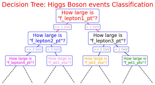
Optional exercise: Draw a decision tree
Here you are an example of how you can build a decision tree by yourself! Try to imagine how the decision tree's growth could proceed in our analysis case and complete it! We give you some hints!
...
import matplotlib.pyplot as plt
%matplotlib inline
fig = plt.figure(figsize=(10, 4))
ax = fig.add_axes([0, 0, 0.8, 1], frameon=False, xticks=[], yticks=[])
ax.set_title('Decision Tree: Higgs Boson events Classification', size=24,color='red')

def text(ax, x, y, t, size=20, **kwargs):
    ax.text(x, y, t,
            ha='center', va='center', size=size,
            bbox=dict( boxstyle='round', ec='blue', fc='w' ), **kwargs)

# Here you are the variables we can use for the training phase:
# --------------------------------------------------------------------------
# High level features:
# ['f_massjj', 'f_deltajj', 'f_mass4l', 'f_Z1mass' , 'f_Z2mass']
# --------------------------------------------------------------------------
# Low level features:
#        [ 'f_lept1_pt','f_lept1_eta','f_lept1_phi', \
#          'f_lept2_pt','f_lept2_eta','f_lept2_phi', \
#          'f_lept3_pt','f_lept3_eta','f_lept3_phi', \
#          'f_lept4_pt','f_lept4_eta','f_lept4_phi', \
#          'f_jet1_pt','f_jet1_eta','f_jet1_phi', \
#          'f_jet2_pt','f_jet2_eta','f_jet2_phi']
#---------------------------------------------------------------------------
text(ax, 0.5, 0.9, "How large is\n\"f_lepton1_pt\"?", 20,color='red')
text(ax, 0.3, 0.6, "How large is\n\"f_lepton2_pt\"?", 18,color='blue')
text(ax, 0.7, 0.6, "How large is\n\"f_lepton3_pt\"?", 18)
text(ax, 0.12, 0.3, "How large is\n\"f_lepton4_pt\"?", 14,color='magenta')
text(ax, 0.38, 0.3, "How large is\n\"f_jet1_eta\"?", 14,color='violet')
text(ax, 0.62, 0.3, "How large is\n\"f_jet2_eta\"?", 14,color='orange')
text(ax, 0.88, 0.3, "How large is\n\"f_jet1_phi\"?", 14,color='green')

text(ax, 0.4, 0.75, ">= 1 GeV", 12, alpha=0.4,color='red')
text(ax, 0.6, 0.75, "< 1 GeV", 12, alpha=0.4,color='red')

text(ax, 0.21, 0.45, ">= 3 GeV", 12, alpha=0.4,color='blue')
text(ax, 0.34, 0.45, "< 3 GeV", 12, alpha=0.4,color='blue')

text(ax, 0.66, 0.45, ">= 2 GeV", 12, alpha=0.4,color='black')
text(ax, 0.79, 0.45, "< 2 GeV", 12, alpha=0.4,color='black')

ax.plot([0.3, 0.5, 0.7], [0.6, 0.9, 0.6], '-k',color='red')
ax.plot([0.12, 0.3, 0.38], [0.3, 0.6, 0.3], '-k',color='blue')
ax.plot([0.62, 0.7, 0.88], [0.3, 0.6, 0.3], '-k')
ax.plot([0.0, 0.12, 0.20], [0.0, 0.3, 0.0], '--k')
ax.plot([0.28, 0.38, 0.48], [0.0, 0.3, 0.0], '--k')
ax.plot([0.52, 0.62, 0.72], [0.0, 0.3, 0.0], '--k')
ax.plot([0.8, 0.88, 1.0], [0.0, 0.3, 0.0], '--k')
ax.axis([0, 1, 0, 1])

fig.savefig('05.08-decision-tree.png')
Random Forest implementation
Now you can start to define a second ML architecture setting the tree construction parameters to fix:
- the assignment of a terminal node to a class;
- the stop splitting of the single tree;
- selection criteria of splits.
Grid Search for Parameter estimation
A machine learning model has two types of parameters. The first type of parameter is the parameters that are learned through a machine learning model while the second type of parameter is the hyperparameter that we pass to the machine learning model.
Normally we set the value for these hyperparameters by hand, as we did for our ANN, and see what parameters result in the best performance. However, randomly selecting the parameters for the algorithm can be exhaustive.
...
import pickle

# Save to file in the current working directory
pkl_filename = "rf_model.pkl"
with open(pkl_filename, 'wb') as file:
    pickle.dump(rfc, file)
Performance evaluation
In this section you will find the following subsections:
- ROC curve and Rates definitions
- Overfitting and test evaluation of an MVA model
If you have the knowledge about these theoretical concepts you may skip it. - Artificial Neural Network performance
- Exercise 1 - Random Forest performance
Here you will re-do the procedure followed for the ANN in order to evaluate the Random Forest performance.
Finally, you will compare the discriminating performance of the two trained ML models.
ROC curve and rates definitions
There are many ways to evaluate the quality of a model’s predictions. In the ANN implementation, we were evaluating the accuracy metrics and losses of the training and validation samples.
...
The AUC is the probability that a classifier will rank a randomly chosen positive instance higher than a randomly chosen negative one. The higher the AUC, the better the performance of the classifier. If the AUC is 0.5, the classifier is uninformative, i.e., it will rank equally a positive or a negative observation.
Other metrics
The precision/purity is the ratio where TPR is the number of true positives and FPR the number of false positives. The precision is intuitively the ability of the classifier not to label as positive a sample that is negative.
...
#Let's import all the metrics that we need later on!
from sklearn.metrics import ConfusionMatrixDisplay,confusion_matrix,accuracy_score , precision_score , recall_score , precision_recall_curve , roc_curve, auc , roc_auc_score
Overfitting and test evaluation of an MVA model
The loss function and the accuracy metrics give us a measure of the overtraining (overfitting) of the ML algorithm. Over-fitting happens when an ML algorithm learns to recognize a pattern that is primarily based on the training (validation) sample and that is nonexistent when looking at the testing (training) set (see the plot on the right side to understand what we would expect when overfitting happens).
Artificial Neural Network performance
Let's see what we obtained from our ANN model training making some plots!
...
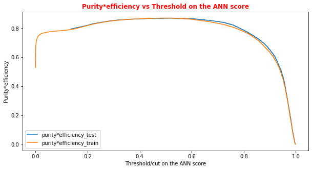
# Plot of the metrics Efficiency x Purity -- ANN
# Looking at this curve we will choose a threshold on the ANN score
# for distinguishing between signal and background events
#plt.plot(t, p[:-1], label='purity_test')
#plt.plot(t_train, p_train[:-1], label='purity_train')
#plt.plot(t, r[:-1], label='efficiency_test')
#plt.plot(t_train, r_train[:-1], label='efficiency_test')
plt.rcParams['figure.figsize'] = (10,5)
plt.plot(t,p[:-1]*r[:-1],label='purity*efficiency_test')
plt.plot(t_train,p_train[:-1]*r_train[:-1],label='purity*efficiency_train')
plt.xlabel('Threshold/cut on the ANN score')
plt.ylabel('Purity*efficiency')
plt.title('Purity*efficiency vs Threshold on the ANN score',fontsize=12,fontweight='bold', color='r')
#plt.tick_params(width=2, grid_alpha=0.5)
plt.legend(markerscale=50)
plt.show()
# Print metrics imposing a threshold for the test sample. In this way the student
# can use later the model's score to discriminate signal and bkg events for a fixing
# score

cut_dnn=0.6

# Transform predictions into a array of entries 0,1 depending if prediction is beyond the
# chosen threshold
y_pred = Y_prediction[:,0]
y_pred[y_pred >= cut_dnn]= 1 #classify them as signal
y_pred[y_pred < cut_dnn]= 0 #classify them as background
y_pred_train = Y_prediction_train[:,0]
y_pred_train[y_pred_train>=cut_dnn]=1
y_pred_train[y_pred_train<cut_dnn]=0

print("y_true.shape",y_true.shape)
print("y_pred.shape",y_pred.shape)
print("w_test.shape",w_test.shape)
print("Y_prediction",Y_prediction)
print("y_pred",y_pred)
...
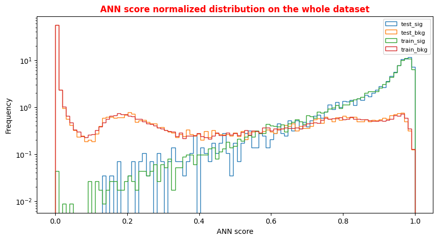
# Normalized Distribution of the ANN score for the whole dataset
# ax = plt.subplot(4, 2, 4)
X = np.linspace(0.0, 1.0, 100) #100 numbers between 0 and 1
plt.rcParams['figure.figsize'] = (10,5)
hist_test_sig = plt.hist(Y_test_sig, bins=X, label='test_sig',histtype='step',log=True,density=1)
hist_test_bkg = plt.hist(Y_test_bkg, bins=X, label='test_bkg',histtype='step',log=True,density=1)
hist_train_sig = plt.hist(Y_train_sig, bins=X, label='train_sig',histtype='step',log=True,density=1)
hist_train_bkg = plt.hist(Y_train_bkg, bins=X, label='train_bkg',histtype='step',log=True,density=1)
plt.xlabel('ANN score')
plt.ylabel('Frequency')
plt.legend( loc='upper right',prop={'size': 8} )
plt.title('ANN score normalized distribution on the whole dataset',fontsize=12,fontweight='bold', color='r')
plt.show()
Exercise 1 - Random Forest performance
Evaluate the performance of the Random Forest algorithm. Hint: use the predict_proba method this time!
In [ ]:
...
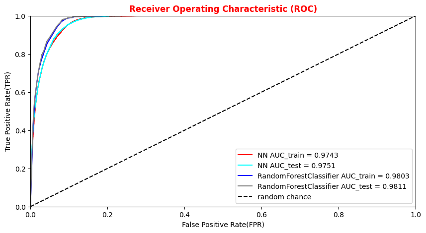
##Superimposition RF and ANN ROC curves
plt.rcParams['figure.figsize'] = (10,5)
plt.plot(fpr_train, tpr_train, color='red', label='NN AUC_train = %.4f' % (roc_auc_train))
plt.plot(fpr, tpr,  color='cyan', label='NN AUC_test = %.4f' % (roc_auc))
#Random Forest 1st method
plt.plot(fpr_train_rf,tpr_train_rf, color='blue', label='RandomForestClassifier AUC_train = %.4f' % (roc_auc_rf_train))
plt.plot(fpr_rf,tpr_rf, color='grey', label='RandomForestClassifier AUC_test = %.4f' % (roc_auc_rf))
#Random Forest 2nd method
#rfc_disp = plot_roc_curve(rfc, X_train_val,Y_train_val,color='brown',ax=ax, sample_weight=w_train )
#rfc_disp = plot_roc_curve(rfc, X_test, Y_test, color='grey',ax=ax, sample_weight=w_test)
#random chance
plt.plot([0, 1], [0, 1], linestyle='--', color='k', label='random chance')
plt.xlim([0, 1.0]) #fpr
plt.ylim([0, 1.0]) #tpr
plt.title('Receiver Operating Characteristic (ROC)',fontsize=12,fontweight='bold', color='r')
plt.xlabel('False Positive Rate(FPR)')
plt.ylabel('True Positive Rate(TPR)')
plt.legend(loc="lower right")
plt.show()
Plot physics observables
We can easily plot the quantities (e.g. ,
,
,
,
) for those events in the datasets which have the ANN and the RF output scores greater than the chosen decision threshold in order to show that the ML discriminators did learned from physics observables!
The subsections of this notebook part are:
...
import matplotlib as mpl
import matplotlib.pyplot as plt

# Define a data frame for low level features
data = df_all.filter(NN_VARS)
X_all   = np.asarray( data.values ).astype(np.float32)
#Use it for evaluating the NN output score for the entire data set
Y_all = model.predict(X_all)
Artificial Neural Network rates fixing an ANN score threshold from data frame
Let's fix a cut (looking at the performance of our models in terms of the previous purity*efficiency metrics plot) on our test statistic (ANN score and RF score) to select mostly VBF Higgs production signal events!
...
ANN score cut chosen:0.6000
TP rate = 0.9494
FP rate = 0.9647
Exercise 2 - Random Forest rates fixing a RF score threshold from dataframe
You can do the same steps for the Random Forest algorithm!
...
RF score cut chosen: 0.6000
TP rate = 0.9812
FP rate = 0.9874
Plot some physical quantities after that the event selection is applied
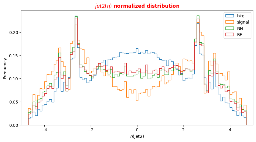
Note that we have not used the low-level features in the training phase of our models, they behaved as spectator variables. We will plot the distribution of events considering their actual label (in the legend signal and background) and the distributions for the two classes that our classifiers have built after having fixed a threshold on their output scores.
...
# Plot Jet2 eta for signal, background and NN/RF selected events
plt.xlabel('$\eta$(Jet2)')
X = np.linspace(-5.,5.,100)
plt.rcParams['figure.figsize'] = (10,5)
df_all['f_jet2_eta'][(df_all['isSignal'] == 0)].plot.hist(bins=X, label='bkg',histtype='step', density=1)
df_all['f_jet2_eta'][(df_all['isSignal'] == 1)].plot.hist(bins=X, label='signal',histtype='step', density=1)
df_sel['f_jet2_eta'].plot.hist(bins=X, label='NN',histtype='step', density=1)
df_sel_rf['f_jet2_eta'].plot.hist(bins=X, label='RF',histtype='step', density=1)
plt.title('$jet2(\eta)$ normalized distribution',fontsize=12,fontweight='bold', color='r')
plt.legend(loc='upper right')
plt.xlim(-5,5)
Optional Exercise 1 - Change the decay channel
Question to students: What happens if you switch to the decay channel? You can submit your model (see the ML challenge below) for this physical process as well!
Optional Exercise 2 - Merge the backgrounds
Question to students: Merge the backgrounds used up to now for the training of our ML algorithms together with the ROOT File named ttH_HToZZ_4L.root. In this case, you will use also the QCD irreducible background. Uncomment the correct lines of code to proceed!
Machine Learning challenge
Once you manage to improve the network (random forest) performances, you can submit your results and participate in our ML challenge. The challenge samples are available in this workspace, but the true labels (isSignal) are removed so that you can't compute the AUC.
...
https://recascloud.ba.infn.it/index.php/s/CnoZuNrlr3x7uPI