...
Grid Search for Parameter estimation
Grid Search for Parameter estimation
A machine learning model has two types of parameters. The first type are is the parameters that are learned through a machine learning model while the second type are the hyperparameters whose value is used to control the learning process.
...
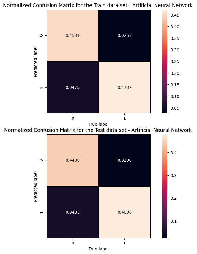
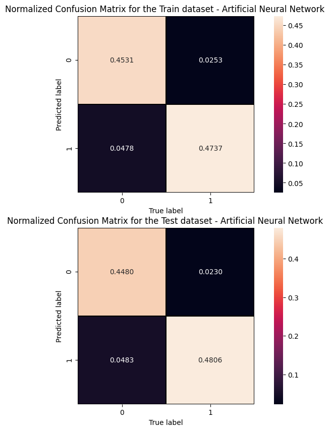
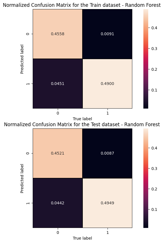
First, we introduce the terms positive and negative referring to the classifier’s prediction, and the terms true and false referring to whether the network prediction corresponds to the observation (the "truth" level). In our Higgs boson binary classification exercise, we can think the negative outcome as the one labeling background (that, in the last sigmoid layer of our network, would mean a number close to 0 - in the Random Forest score would mean a number equals to zero), and the positive outcome the outcome as the one labeling signal (that, in the last sigmoid layer of our network, would mean a number close to 1 - random forest score equals to zero).
...
Cut/Threshold on the ANN output : 0.6000 Confusion matrix ANN
An alternative way to check overfitting, and choosing correctly a threshold for selecting signal events, is plotting signal and background ANN predictions for the training and test datasets. If the distributions are quite similar it means that the algorithm learned how to generalize!
For measuring quantitatively the overfitting one can perform a Kolmogorov-Smirnov test that we will not implement here.
...
Cut/Threshold on the Random Forest output : 0.6000

##Superimposition RF and ANN ROC curves
plt.rcParams['figure.figsize'] = (10,5)
plt.plot(fpr_train, tpr_train, color='red', label='NN AUC_train = %.4f' % (roc_auc_train))
plt.plot(fpr, tpr,  color='cyan', label='NN AUC_test = %.4f' % (roc_auc))
#Random Forest 1st method
plt.plot(fpr_train_rf,tpr_train_rf, color='blue', label='RandomForestClassifier AUC_train = %.4f' % (roc_auc_rf_train))
plt.plot(fpr_rf,tpr_rf, color='grey', label='RandomForestClassifier AUC_test = %.4f' % (roc_auc_rf))
#Random Forest 2nd method
#rfc_disp = plot_roc_curve(rfc, X_train_val,Y_train_val,color='brown',ax=ax, sample_weight=w_train )
#rfc_disp = plot_roc_curve(rfc, X_test, Y_test, color='grey',ax=ax, sample_weight=w_test)
#random chance
plt.plot([0, 1], [0, 1], linestyle='--', color='k', label='random chance')
plt.xlim([0, 1.0]) #fpr
plt.ylim([0, 1.0]) #tpr
plt.title('Receiver Operating Characteristic (ROC)',fontsize=12,fontweight='bold', color='r')
plt.xlabel('False Positive Rate(FPR)')
plt.ylabel('True Positive Rate(TPR)')
plt.legend(loc="lower right")
plt.show()
...