Author(s)
| Name | Institution | Mail Address | Social Contacts |
|---|---|---|---|
| Camilla Scapicchio | University of Pisa, INFN Sezione di Pisa | Linkedin: Camilla Scapicchio | |
| Francesca Lizzi | University of Pisa, INFN Sezione di Pisa | francesca.lizzi@sns.it |
How to Obtain Support
General Information
| ML/DL Technologies | CNN (ResNet) |
|---|---|
| Science Fields | Medical Physics |
| Difficulty | Low |
| Language | English |
| Type | Fully annotated and runnable |
Software and Tools
| Programming Language | Python |
|---|---|
| ML Toolset | Keras, Tensorflow |
| Additional libraries | sklearn, pandas, OpenCv |
| Suggested Environments | INFN-Cloud VM, bare Linux Node, Google CoLab |
Needed datasets
| Data Type | Preprocessed Mammographic Images |
|---|---|
| Data Source | Examples of test images on GitHub repository: https://github.com/camillascapicchio/MLINFN-CNNBreastDensityClassifier-Explainability |
Short Description of the Use Case
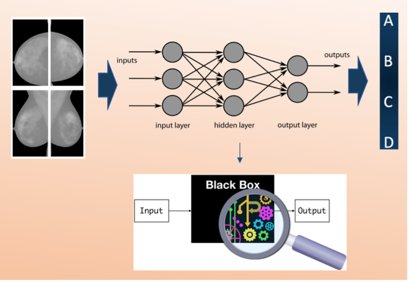
Deep neural network explainability is a critical issue in Artificial Intelligence (AI). In this use case, we develop a method to explain a deep Residual Convolutional Neural Network able to automatically classify mammograms into breast density classes.
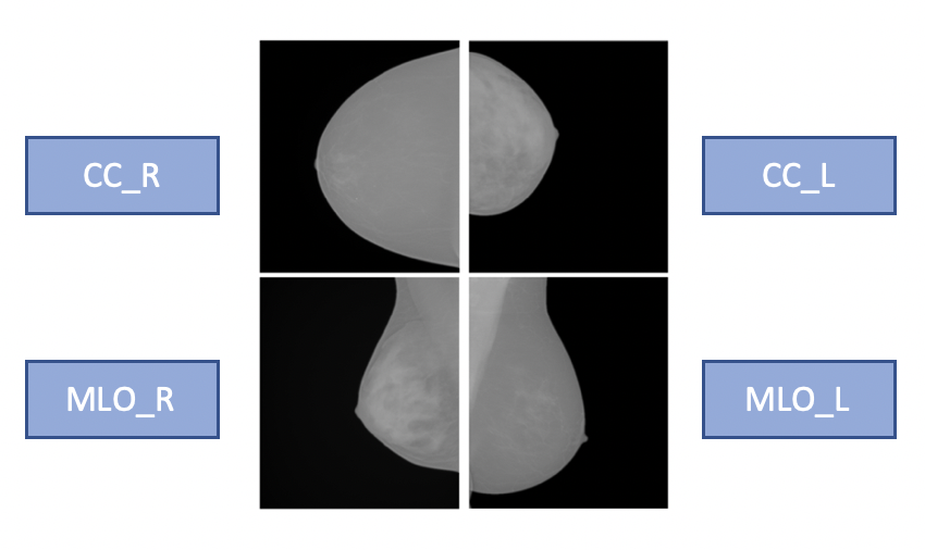
Breast density is defined as the amount of dense tissue in the breast, visible on a mammogram, compared to the amount of fatty tissue. The denser glandular tissue attenuates radiation more with respect to fat tissue that shows up darker in the mammographic image because less attenuating. Breast density itself is an independent risk factor for breast cancer. Each mammographic exam of each subject consists of 4 separate images which are the 4 different projections acquired by the mammographic system, Cranio-Caudal for Right and Left breasts (CC_R, CC_L) and Medio-Lateral-Oblique for Right and Left breasts (MLO_R, MLO_L).
Each exam is evaluated by a radiologist and assigned to a density class label, following the standard reported in the BIRADS (Breast Imaging Reporting and Data System) Atlas: entirely fatty (A), scattered areas of fibroglandular density (B), heterogeneously dense (C) and extremely dense (D). A, B, C and D are the 4 class labels in our classification problem, and the classification made by the radiologist is our ground truth.
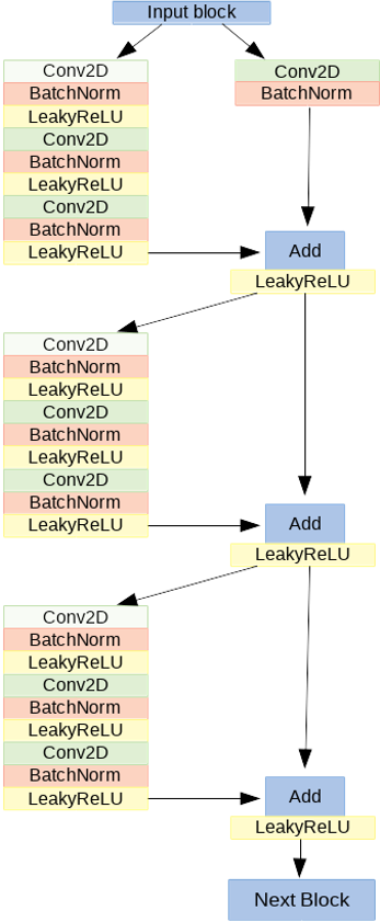
We want to reproduce this classification with a 2D Convolutional Neural Network (CNN) with a residual architecture (ResNet model). It is made of 41 convolutional layers, organized in residual blocks. It has about 2 million learnable parameters. The input block consists of a convolutional layer, a batch normalization layer, a leakyReLU as activation function and a 2D-max pooling. The output of this block has been fed into a series of four blocks, each made of 3 residual modules. In the figure, the architecture of one of the four blocks is shown:
It is too expensive to train this model on the 4 projections simultaneously in terms of GPUs RAM. Therefore, we train four different CNNs per projection. The classification scores of the last layers of each CNN will be averaged to produce a label that takes into account all the images related to a single subject. It is suggested to train the network on at least about 1000 images to obtain a good performance. We obtained the following performance:
accuracy | 0.81 |
recall | 0.81 |
precision | 0.80 |
with a private dataset annotated by a radiologist with one of the four BIRADS density classes (A, B, C, D). The images have been acquired with GE Senograph DS imaging systems. The data were also randomly split into a training set (80%), a validation set (10%) and a test set (10%). Before using them for the training, the images underwent some preprocessing steps:
- Conversion from DICOM file to PNG.
- 8 bits conversion, as Keras does not support 12 or 16 bits images.
- Background removal, the images are cropped at the breast skin edge line.
- Pectoral muscle removal in MLO projections. As it is dense tissue, it could be a source of confusion for a density classifier. It was segmented and replaced with the mean gray value of the breast
Some examples of these preprocessed mammographic images are available as test images on GitHub repository:
The aim of this tutorial is to share our knowledge to allow you to use your own dataset, which could be fundamental to evaluate the robustness of the model.
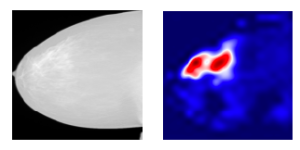
After training, testing and evaluating the classification performance of the CNN through the figures of merit of accuracy, recall and precision, the second step is to check if the network is reliable and understand the reasons behind its predictions, as being a deep neural network, they remain quite unclear. This means that we want to verify if the classification is made by “looking at” what we expected, i.e. the dense regions in the mammogram. This analysis of explainability could be implemented through an off-line (applied after training the model, without altering its architecture) visualization technique. This technique aims to identify which discriminative pixels in the image influence the final prediction.
We use the visualize_cam utility function, provided by Keras, to generate a gradient-based Class Activation Map, which is an image indicating the input regions whose change would most contribute towards maximizing the output. This function is based on the grad-CAM specific technique. The Grad-CAM LcGrad-CAM is a weighted combination of forward activation maps, followed by a ReLU:
The neuron importance weight ack highlights the "importance" of feature map k for a target class c. To obtain these weights, we first compute the gradient of the score for class c, yc, with respect to feature map activations Ak of a convolutional layer, i.e. ∂yc/∂Ak. Then these gradients flowing back are global-average-pooled over the width and height dimensions (indexed by i and j respectively). The places where the gradient is large let us exactly define the region that has a large impact on the final score decision. Thus, we obtain a heatmap that indicates which areas of an image are being used by the model for discrimination among classes.
Together with high performance results, explainability is fundamental to assess trust in the model, to make it a potential application in clinical practice.
How to execute it
The software package, which allows an end-to-end approach, from the building and training of the network to the obtaining and visualization of the heatmaps to explain the network, is available and fully explained in a GitHub repository: https://github.com/camillascapicchio/MLINFN-CNNBreastDensityClassifier-Explainability
You need Jupyter notebook as well as all the Python packages necessary to run it.
In the folder “myproject” you can find all the useful scripts:
1) The first script Train_ResNet.py is the script to train the CNN. Since a good performance requires a training on at least 1000 images, the training of each network requires at least 1xGPU nVidia Tesla K80 as hardware and the training requires about 24h to be completed.
2) The second script in python Prediction_ResNet.py is to test the model. It can also be run locally on a common hardware but paying attention to use the same virtual environment used for the training, because you need the same version of the packages to be sure that the algorithm is compatible and reliable.
3-4) The third and fourth scripts Figure_merit.ipynb and ClassActivationMaps.ipynb are Jupiter notebooks, the first is to obtain the figures of merit, the second to generate the Class Activation Maps. They can be run on Google CoLab or you can clone the GitHub repo and execute the notebook locally.
The software package is designed for a double purpose:
- since our private dataset cannot be shared and given the difficulty in finding public medical imaging data in mammography, we share the software to encourage other users to use their own datasets. Therefore, if the user has his own training dataset and the required hardware available, the training can be run. The details of our dataset and our results can be used as a benchmark. This could be fundamental to evaluate the robustness of the model on a different dataset and check the reproducibility of the algorithms.
- the other option, if a huge dataset and the hardware are not available, is to use this software package as a tutorial in the field of Medical Physics, useful to learn how to build a CNN classifier, test it, and especially generate the activation maps to understand the reasons behind the predictions, for which a standard method is currently non-existent. In this case, the first training script can be used just to visualize how the model is built without running it. While the next scripts, from the test of the model to the maps generation (from 2 to 4), can be run by using the few examples of preprocessed mammographic images we uploaded on GitHub repository, which can be used as test images, together with some files containing the weights of a pre-trained model, to test the functioning of the software.
Annotated Description
- Train_ResNet.py: this is the first script to execute if you want to train the CNN ResNet model from scratch. You may train the network four times, one per projection. You can use your own dataset as training set. It should consist of at least about 1000 images and it should be divided in 4 different folders (CC_R, CC_L, MLO_L, MLO_R) and each folder divided into 4 sub-folders, one per class (A, B, C, D). In "CC_R_model" directory we saved the output of a training as an example.
- Prediction_ResNet.py: this is the script to test the saved trained model on new images. It is suggested to use your own test set also for testing. The test set of images should be organized in folders as the training set. If you don't have enough images to train the model but you just want to test it, you can use a pre-trained model ('weights-improvement-46-0.80.h5') saved in the folder "CC_R_model".
- Figure_merit.ipynb: this is the script to obtain the metrics, the final figures of merit to evaluate the classification performance on the test set. You need the .txt files, obtained with the script "Prediction_ResNet.py" and containing the prediction outcomes, as input. We uploaded "predictions_mlor.txt, predictions_ccr.txt, predictions_mlol.txt, predictions_ccl.txt" files in folder "Prediction", obtained from a pre-trained and tested ResNet model to use them as examples.
- ClassActivationMaps.ipynb: this is the script to obtain the Class Activation Maps based on the Grad-CAM technique. You can use the test images we uploaded as example in the folder “TestSet”, they are just one image per class for each projection. You can use them and the pre-trained model in the folder "CC_R_model" to try the script as a tutorial the first time. Then, you can execute the script on your own larger dataset and on your trained model to obtain the maps in your specific case.
References
Here you can find a more detailed description of the ResNet model architecture: https://link.springer.com/chapter/10.1007/978-3-030-29930-9_3
Here you can find a more detailed description of the Grad-CAM technique: https://openaccess.thecvf.com/content_iccv_2017/html/Selvaraju_Grad-CAM_Visual_Explanations_ICCV_2017_paper.html


