...
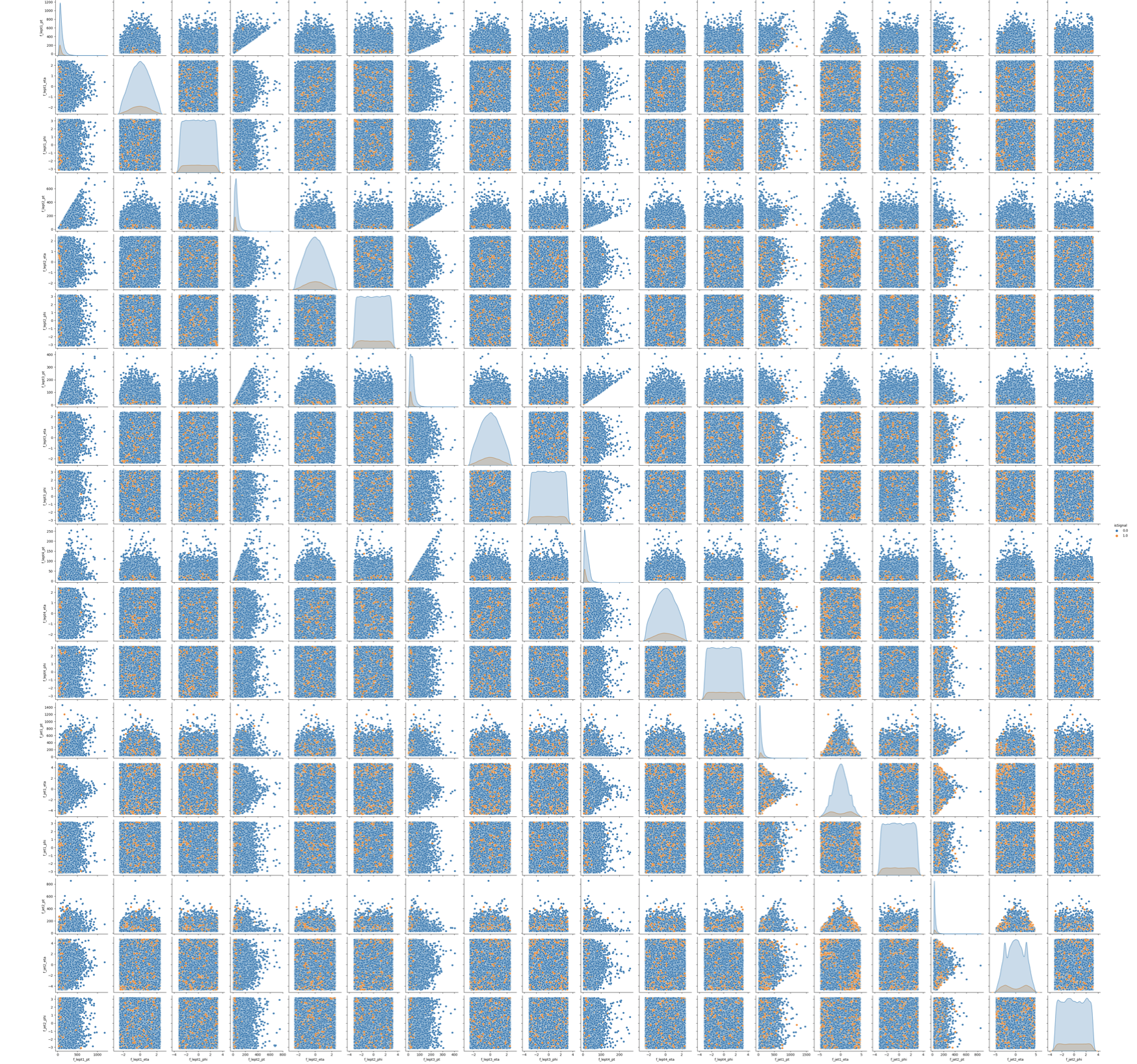
# It will take a while (1 hour). Skip it!
# We leave you the output of this code cell using a .png format

# NN_VARS = ['f_lept1_pt','f_lept1_eta','f_lept1_phi', \
#           'f_lept2_pt','f_lept2_eta','f_lept2_phi', \
#           'f_lept3_pt','f_lept3_eta','f_lept3_phi', \
#           'f_lept4_pt','f_lept4_eta','f_lept4_phi', \
#           'f_jet1_pt','f_jet1_eta','f_jet1_phi', \
#           'f_jet2_pt','f_jet2_eta','f_jet2_phi', 'isSignal']
# sns.pairplot( data=df_all.filter(NN_VARS), hue='isSignal' , kind='scatter', diag_kind='auto' );
# Filter dataframe leaving just the Neural Network and Random Forest input variables

NN_VARS= ['f_massjj', 'f_deltajj', 'f_mass4l', 'f_Z1mass' , 'f_Z2mass']
# NN_VARS = [ 'f_lept1_pt','f_lept1_eta','f_lept1_phi', \
#          'f_lept2_pt','f_lept2_eta','f_lept2_phi', \
#          'f_lept3_pt','f_lept3_eta','f_lept3_phi', \
#          'f_lept4_pt','f_lept4_eta','f_lept4_phi', \
#          'f_jet1_pt','f_jet1_eta','f_jet1_phi', \
#          'f_jet2_pt','f_jet2_eta','f_jet2_phi']

df_input  = df_all.filter(NN_VARS)
df_target = df_all.filter(['isSignal']) # flag
df_weights = df_all.filter(['f_weight'])
# the weights are also important to be given as input to the training

# Transform dataframes to numpy arrays of float32
# (X->NN input , Y->NN target output , W-> event weights)

NINPUT=len(NN_VARS)
print("Number NN input variables=",NINPUT)
print("NN input variables=",NN_VARS)
X  = np.asarray( df_input.values ).astype(np.float32)
Y  = np.asarray( df_target.values ).astype(np.float32)
W  = np.asarray( df_weights.values ).astype(np.float32)
print(X.shape)
print(Y.shape)
print(W.shape)
print('\n')
Number NN input variables= 5
NN input variables= ['f_massjj', 'f_deltajj', 'f_mass4l', 'f_Z1mass', 'f_Z2mass']
(114984, 5)
(114984, 1)
(114984, 1)
Dividing the data into testing and training data set
You can split now the datasets into two parts (one for the training and validation steps and one for testing phase).
Question to students: Have a look to the parameter setting test_size. Why did we choose that small fraction of events to be used for the testing phase?
# Classical way to proceed, using a scikit-learn algorithm:
# X_train_val, X_test, Y_train_val , Y_test , W_train_val , W_test =
# train_test_split(X, Y, W , test_size=0.2,shuffle=None,stratify=None )

# Alternative way, the one that we chose in order to study the model's performance
# with ease (with an analogous procedure used by TMVA in ROOT framework)
# to keep information about the flag isSignal in both training and test steps.

size= int(len(X[:,0]))
test_size = int(0.2*len(X[:,0]))
print('X (features) before splitting')
print('\n')
print(X.shape)
print('X (features) splitting between test and training')
X_test= X[0:test_size+1,:]
print('Test:')
print(X_test.shape)
X_train_val= X[test_size+1:len(X[:,0]),:]
print('Training:')
print(X_train_val.shape)
print('\n')
print('Y (target) before splitting')
print('\n')
print(Y.shape)
print('Y (target) splitting between test and training ')
Y_test= Y[0:test_size+1,:]
print('Test:')
print(Y_test.shape)
Y_train_val= Y[test_size+1:len(Y[:,0]),:]
print('Training:')
print(Y_train_val.shape)
print('\n')
print('W (weights) before splitting')
print('\n')
print(W.shape)
print('W (weights) splitting between test and training ')
W_test= W[0:test_size+1,:]
print('Test:')
print(W_test.shape)
W_train_val= W[test_size+1:len(W[:,0]),:]
print('Training:')
print(W_train_val.shape)
print('\n')
X (features) before splitting


(114984, 5)
X (features) splitting between test and training
Test:
(22997, 5)
Training:
(91987, 5)


Y (target) before splitting


(114984, 1)
Y (target) splitting between test and training
Test:
(22997, 1)
Training:
(91987, 1)


W (weights) before splitting


(114984, 1)
W (weights) splitting between test and training
Test:
(22997, 1)
Training:
(91987, 1)
Description of the Artificial Neural Network (ANN) model and KERAS API
In this section you will find the following subsections:
- Introduction to the Neural Network algorithm
If you have the knowledge about ANN you may skip it. - Usage of Keras API: basic concepts
Here you find concepts that are useful for the ANN implementation using KERAS API (callfunctions, metrics etc.).
There are three ways to create Keras models:
- The Sequential model, which is very straightforward (a simple list of layers), but is limited to single-input, single-output stacks of layers (as the name gives away).
- The Functional API, which is an easy-to-use, fully-featured API that supports arbitrary model architectures. For most people and most use cases, this is what you should be using. This is the Keras "industry strength" model. We will use it.
- Model subclassing, where you implement everything from scratch on your own. Use this if you have complex, out-of-the-box research use cases.
Introduction to the Neural Network algorithm
A Neural Network (NN) is a biology inspired analytical model, but not bio-mimetic one. It is formed by a network of basic elements called neurons or perceptrons (see the picture below), which receive an input, change their state according to the input and produce an output.
The neuron/perceptron concept
The perceptron, while it has a simple structure, has the ability to learn and solve very complex problems.
- It takes the inputs which are fed into the perceptrons, multiplies them by their weights, and computes the sum. In the first iteration the weights are set randomly.
- It adds the number one, multiplied by a “bias weight”. This makes it possible to move the output function of each perceptron (the activation function) up, down, left and right on the number graph.
- It feeds the sum through the activation function in a simple perceptron system, the activation function is a step function.
- The result of the step function is the neuron output.
Neural Network Topologies
A Neural Networks (NN) can be classified according to the type of neuron interconections and the flow of information.
Feed Forward Networks
A feedforward NN is a neural network where connections between the nodes do not form a cycle. In a feed forward network information always moves one direction, from input to output, and it never goes backwards. Feedforward NN can be viewed as mathematical models of a func5on .
Recurrent Neural Network
A Recurrent Neural Network (RNN) is a neural network that allows connections between nodes in the same layer, with themselves or with previous layers.
Unlike feedforward neural networks, RNNs can use their internal state (memory) to process sequential input data.
Dense Layer
A Neural Network layer is called a dense layer to indicate that it’s fully connected. Information about the Neural Network architectures see: https://www.asimovinstitute.org/neural-network-zoo/
Artificial Neural Network
The discriminant output is computed by combining the response of multiple nodes, each representing a single neuron cell. Nodes are arranged into layers.
In an ANN the input variable values are passed to a first input layer, whose output is passed as input to the next layer, and so on.
The last output layer is usually constituted by a single node that provides the discriminant output. Intermediate layers between the input and the output layers are called hidden layers. Usually if a Neural Network as more than one hidden layer is called Deep Neural Network and is able to do by itself the feature extraction (it becomes a Deep Learning algorithm).
Such a structure is also called Feedforward Multilayer Perceptron (MLP, see the picture).
The output of the node of the
layers is computed as weighted average of the input variables, with weights that are subject to optimization via training.
The activation layer filters out the output , using an activation function. It converts the output of a given layer before passing on the information to consecutive layers. It can be a sigmoid, arctangent, step function (new functions as ReLu,SeLu) because they mimic a learning curve.
Then a bias or threshold parameter is applied. This bias accounts for the random noise, in the sense that it measures how well the model fits the training set (how much the model is able to correctly predict the known outputs of the training examples.) The output of a given node is:
.
Supervised Learning: the loss function
In order to train the neural network, a further function is introduced in the model, the loss (cost) function that quantifies the error between the NN output and the desired target output.The choice of the loss function is directly related to the activation function used in the output layer !
If we have binary targets we use the Cross Entropy Loss:
.
During training we optimize the loss function, i.e. reduce the error between actual and predicted values. Since we deal with a binary classification problem, the can take on just two values,
(for hypothesis
) and
(for hypothesis
).
A popular algorithm to optimize the weights, consists in iteratively modifying the weights afer each training observation or after a bunch of training observation by doing a minimization of the loss function.
The minimization usually proceeds via the so-called Stochastic Gradient Descent (SGD) which modifies weight at each iteration according to the following formula: .
Other more complex optimization algorithms are available in KERAS API.
More info: https://keras.io/api/optimizers/.
Metrics
A metric is a function that is used to judge the performance of your model.
Metric functions are similar to loss functions, except that the results from evaluating a metric are not used when training the model. Note that you may use any loss function as a metric.