Author(s)
| Name | Institution | Mail Address | Social Contacts |
|---|---|---|---|
| Brunella D'Anzi | INFN Sezione di Bari | brunella.d'anzi@cern.ch | Skype: live:ary.d.anzi_1; Linkedin: brunella-d-anzi |
| Nicola De Filippis | INFN Sezione di Bari | nicola.defilippis@ba.infn.it | |
Domenico Diacono | INFN Sezione di Bari | domenico.diacono@ba.infn.it | |
| Walaa Elmetenawee | INFN Sezione di Bari | walaa.elmetenawee@cern.ch | |
| Giorgia Miniello | INFN Sezione di Bari | giorgia.miniello@ba.infn.it | |
| Andre Sznajder | Rio de Janeiro State University | sznajder.andre@gmail.com |
How to Obtain Support
| brunella.d'anzi@cern.ch,giorgia.miniello@ba.infn.it | |
| Social | Skype: live:ary.d.anzi_1; Linkedin: brunella-d-anzi |
General Information
| ML/DL Technologies | Artificial Neural Networks (ANNs), Random Forests (RFs) |
|---|---|
| Science Fields | High Energy Physics |
| Difficulty | Low |
| Language | English |
| Type | fully annotated and runnable |
Software and Tools
| Programming Language | Python |
|---|---|
| ML Toolset | |
| Additional libraries | uproot, NumPy, pandas,h5py,seaborn,matplotlib |
| Suggested Environments | Google's Colaboratory |
Needed datasets
| Data Creator | CMS Experiment |
|---|---|
| Data Type | Simulation |
| Data Size | 2 GB |
| Data Source | Cloud@ReCaS-Bari |
Short Description of the Use Case
Introduction to the statistical analysis problem
In this exercise, you will perform a binary classification task using Monte Carlo simulated samples representing the Vector Boson Fusion (VBF) Higgs boson production in the four-lepton final state signal and its main background processes at the Large Hadron Collider (LHC) experiments. Two Machine Learning (ML) algorithms will be implemented: an Artificial Neural Network (ANN) and a Random Forest (RF).
- You will learn how a multivariate analysis algorithm works (see the below introduction) and more specifically how a Machine Learning model must be implemented;
- you will acquire basic knowledge about the *Higgs boson physics* as described by the Standard Model. During the exercise you will be invited to plot some physical quantities in order to understand what is the underlying Particle Physics problem;
- you will be invited to *change hyperparameters* of the ANN and the RF parameters to understand better what are the consequences in terms of the models' performances;
- you will understand that the choice of the *input variables* is a key task of a Machine Learning algorithm since an optimal choice allows achieving the best possible performances;
- moreover, you will have the possibility of changing the background datasets, the decay channels of the final state particles, and seeing how the ML algorithms' performance changes.
Multivariate Analysis and Machine Learning algorithms: basic concepts
Multivariate Analysis algorithms receive as input a set of discriminating variables. Each variable alone does not allow to reach an optimal discrimination power between two categories (we will focus on a binary task in this exercise). Therefore the algorithms compute an output that combines the input variables.
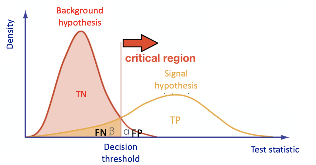
This is what every Multivariate Analysis (MVA) discriminator does. The discriminant output, also called discriminator, score, or classifier, is used as a test statistic and is then adopted to perform the signal selection. It could be used as a variable on which we decide to cut in a hypothesis test.
In particular, Machine Learning tools are models that have enough capacity to define their own internal representation of the data to accomplish a task: learning from data and make predictions without being explicitly programmed to do so.
In the case of binary classification, firstly the algorithm is trained with two datasets:
- one that contains events distributed according to the null (in our case signal, there exists another convention in actual physics analysis) hypothesis H0 ;
- another data set according to the alternative (in our case background) hypothesis H1.
and it must learn how to classify new datasets (the test dataset in our case).
This means that we have the same set of features (random variables) with their own distribution on the H0 and H1 hypotheses.
To obtain a good ML classifier with high discriminating power, we will follow the following steps:
- Training (learning): a discriminator is built by using all the input variables. Then, the parameters are iteratively modified by comparing the discriminant output to the true label of the dataset (supervised machine learning algorithms, we will use two of them). This phase is crucial, one should tune the input variables and the parameters of the algorithm!
- Alternatively, algorithms that group and find patterns in the data according to the observed distribution of the input data are called unsupervised learning.
- A good habit is training multiple models with various hyperparameters on a “reduced” training set ( i.e. the full training set minus the so-called validation set), and then select the model that performs best on the validation set. If you have the possibility of having more than one validation set, you can do a so-called cross-validation check (we will do it on the RF algorithm).
- Once, the validation process is over, you re-train the best model on the full training set (including the validation set), and this gives you the final model
- Alternatively, algorithms that group and find patterns in the data according to the observed distribution of the input data are called unsupervised learning.
- Test: once the training has been performed, the discriminator score is computed in a separated, independent dataset for both H0 and H1.
- An overfitting check is performed between test and training classifier and their performances are computed (e.g. in terms of ROC curves).
- If the test fails, and the performances of the test and training are different, it is a symptom of overtraining and the model is not good!
A description of the Artificial Neural Network and Random Forest algorithms is inserted in the notebook itself.
Particle Physics basic concepts: the Standard Model and the Higgs boson
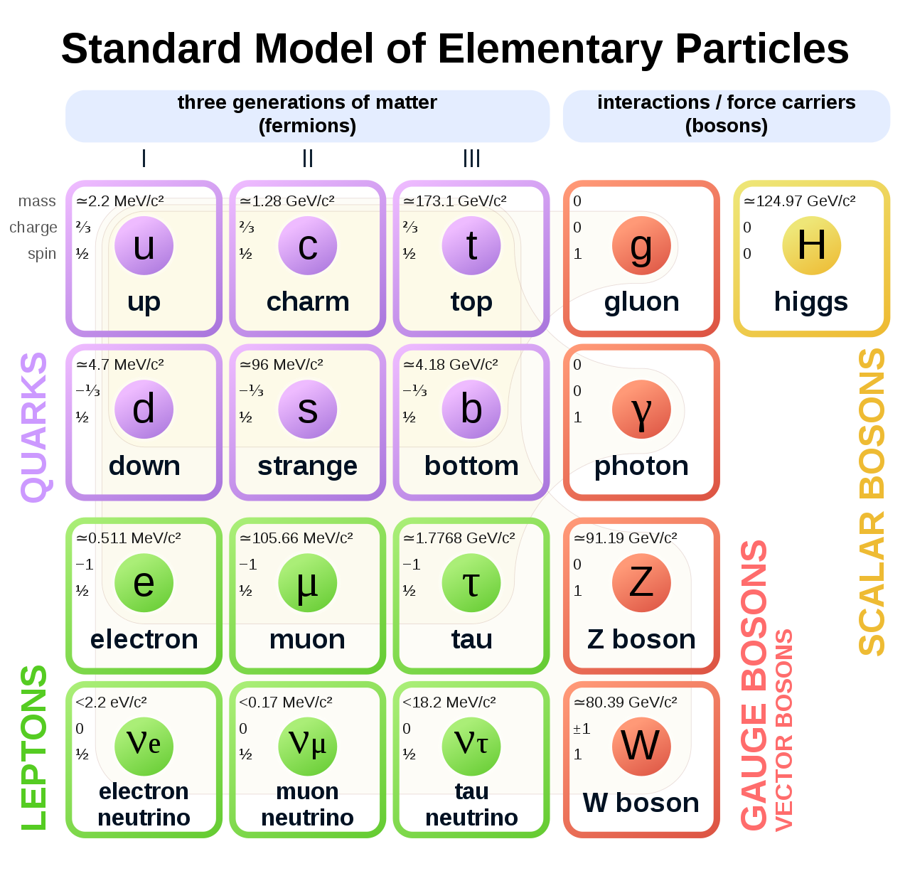
The Standard Model of elementary particles represents our knowledge of the microscopic world. It describes the matter constituents (quarks and leptons) and their interactions (mediated by bosons), which are the electromagnetic, the weak, and the strong interactions.
Among all these particles, the Higgs boson still represents a very peculiar case. It is the second heaviest known elementary particle (mass of 125 GeV) after the top quark (175 GeV).
The ideal tool for measuring the Higgs boson properties is a particle collider. The Large Hadron Collider (LHC), situated nearby Geneva, between France and Switzerland, is the largest proton-proton collider ever built on Earth. It consists of a 27 km circumference ring, where proton beams are smashed at a center-of-mass energy of 13 TeV (99.999999% of the speed of light). At the LHC, 40 Million collisions / second occurs, providing an enormous amount of data. Thanks to these data, ATLAS and CMS experiments discovered the missing piece of the Standard Model, the Higgs boson, in 2012.
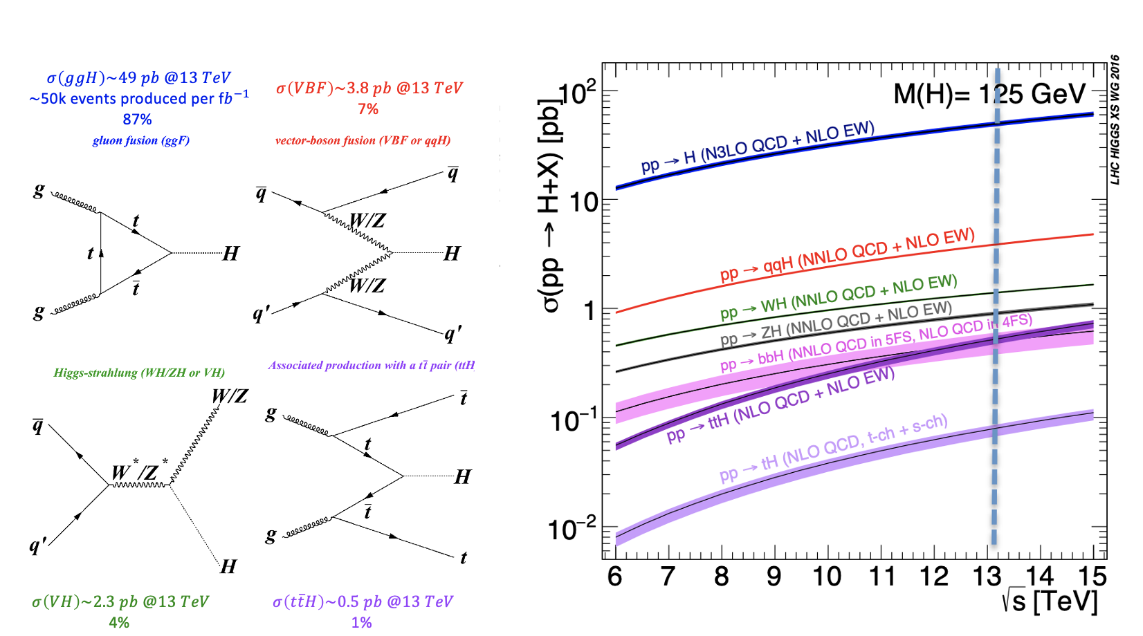
During a collision, the energy is so high that protons are "broken" into their fundamental components, i.e. quarks and gluons, that can interact together, producing particles that we don't observe in our everyday life, such as the Higgs boson. The production of a Higgs boson via a vector boson fusion (VBF) mechanism is, by the way, a relatively "rare" phenomenon, since there are other physical processes that occur way more often, such as those initiated by strong interaction, producing the Higgs boson by the so-called gluon-gluon fusion (ggH) production process. In High Energy Physics, we speak about the cross-section of a physics process. We say that the Higgs boson production via the vector boson fusion mechanism has a smaller cross-section than the production of the same boson (scalar particle) via the ggH mechanism.
The experimental consequence is that distinguishing the two processes, which are characterized by the decay products, can be extremely difficult, given that the latter phenomenon has a way larger probability to happen. In the exercise, we will propose to merge different backgrounds to be distinguished from the signal events.
Experimental signature of the Higgs boson in a particle detector
Let's first understand what are the experimental signatures and how the LHC's detectors work. As an example, this is a sketch of the Compact Muon Solenoid (CMS) detector.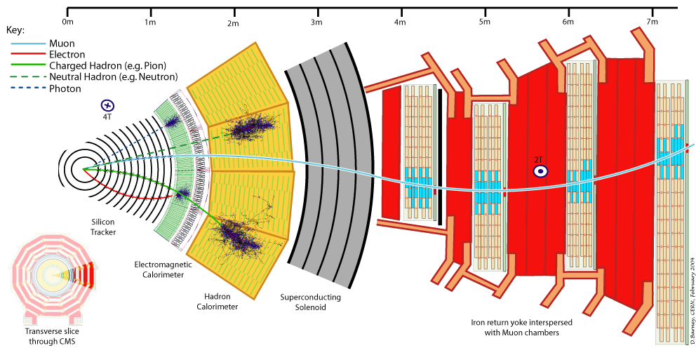
A collider detector is organized in layers: each layer is able to distinguish and measure different particles and their properties. For example, the silicon tracker detects each particle that is charged. The electromagnetic calorimeter detects photons and electrons. The hadronic calorimeter detects hadrons (such as protons and neutrons). The muon chambers detect muons (that have a long lifetime and travel through the inner layers).
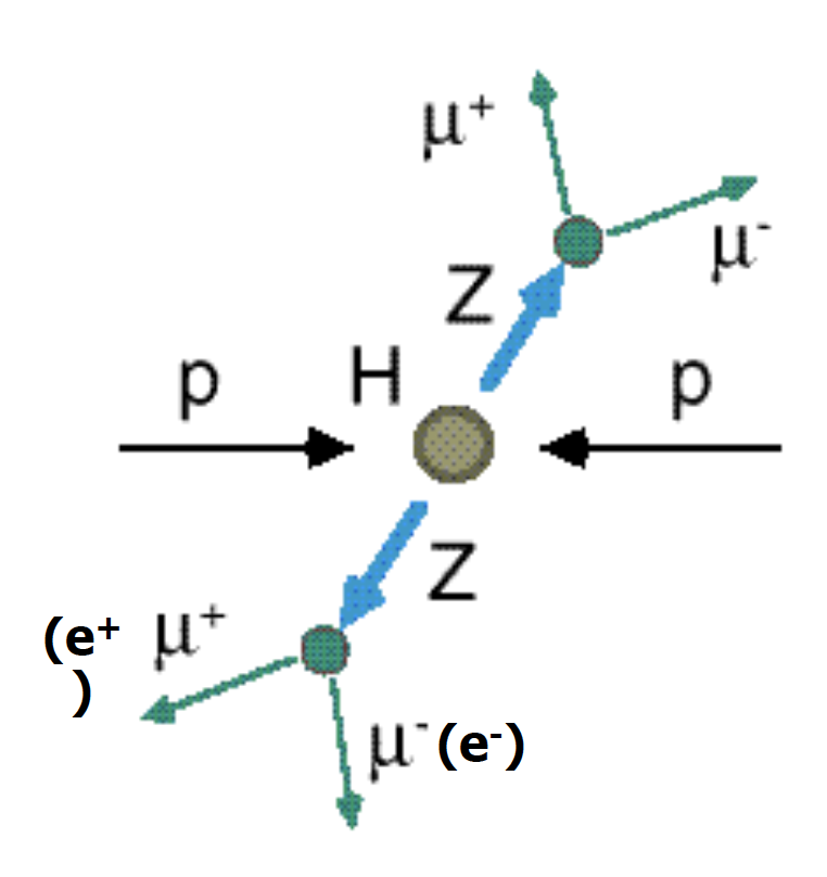
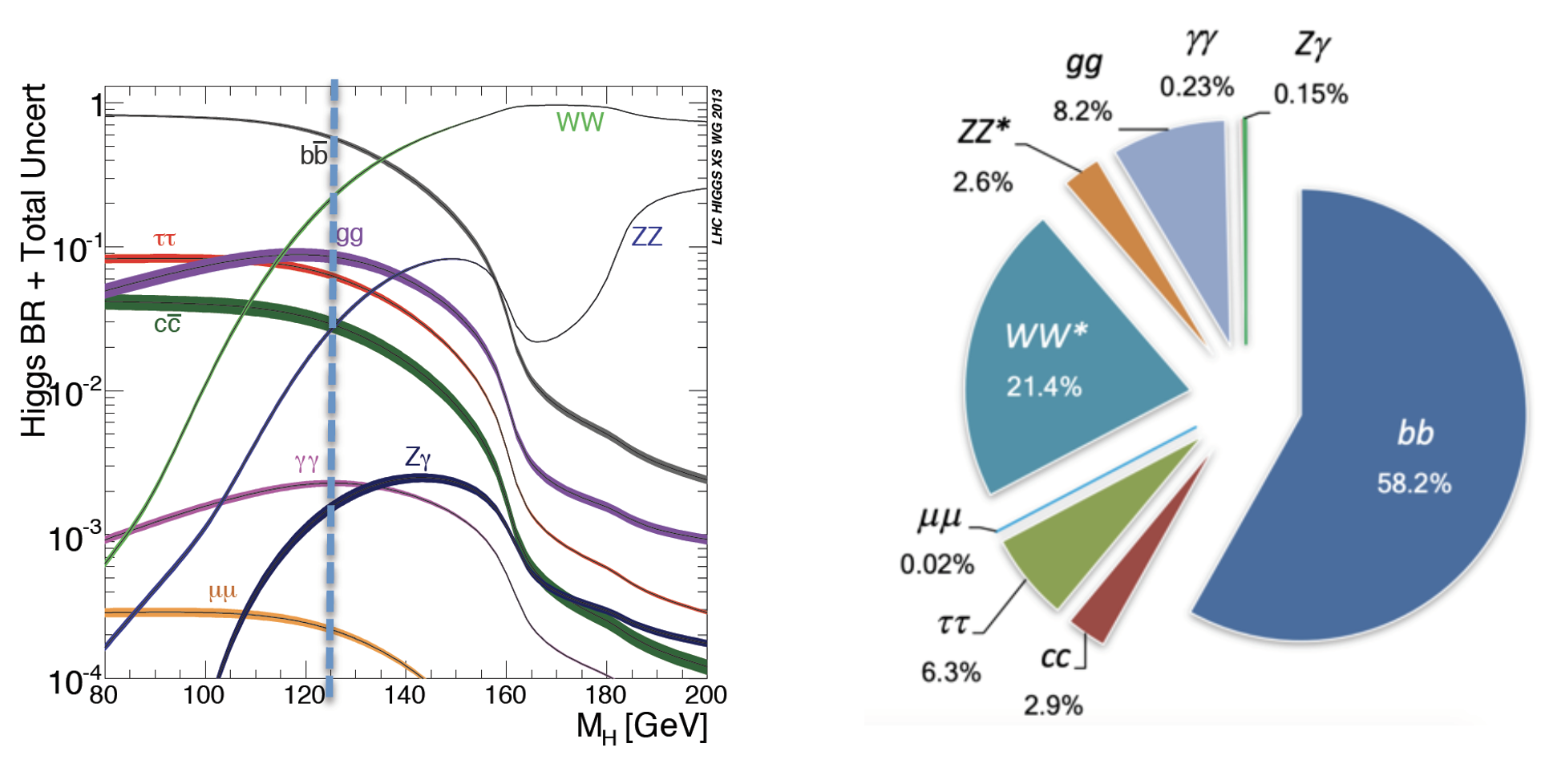
Our physics problem consists of detecting the so-called golden channel H→ ZZ*→ l+ l- l'+ l'- which is one of the possible Higgs boson's decays: its name is due to the fact that it has the clearest and cleanest signature of all the possible Higgs boson decay modes. The decay chain is sketched here: the Higgs boson decays into Z boson pairs, which in turn decay into a lepton pair (in the picture, muon-antimuon or electron-positron pairs). In this exercise, we will use only datasets concerning the 4mu decay channel and the datasets about the 4e channel are given to you to be analyzed as an optional exercise. At the LHC experiments, the decay channel 2e2mu is also widely analyzed.
Data exploration
In this exercise we are mainly interested in the following ROOT files (you may look at the web page ROOT file if you would like to learn more about which kind of objects you can store in them):
- VBF_HToZZTo4mu.root;
- GluGlueHtoZZTo4mu.root;
- ZZto4mu.root.
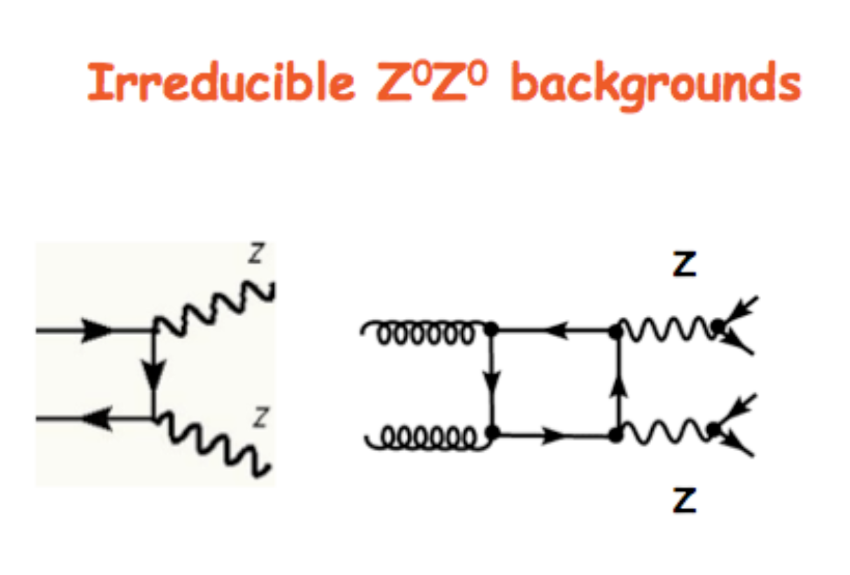
The VBF ROOT file contains the Higgs boson production (mass of 125 GeV) via the Vector Boson Fusion (VBF) mechanism (qqH) signal events - that we want to discriminate from the so-called Gluon Gluon Fusion (ggH) Higgs production events and the QCD process ZZ → 4mu which are both irreducible backgrounds (see the Feynmann diagram in the pictures and the cross-sections/branching ratios expected for Higgs boson production processes and its decay channels).
The processes are characterized by the same final-state particles but we can use the value of multiple variables, such as kinematic properties of the particles, for classifying data into the two categories, signal, and background. The first one is the statistically less probable process that results in producing the Higgs boson at the Large Hadron Collider (LHC) experiments and it is still understudies by the CMS collaboration.
 In order to train our Machine Learning algorithms, we will look at the decay products of our physics problem. In our case we going to deal with:
- electrically-charged leptons (electrons or muons, denoted l)
- particle jets (collimated streams of particles originating from quarks or gluons, denoted j).
For each object, several kinetic variables are measured:
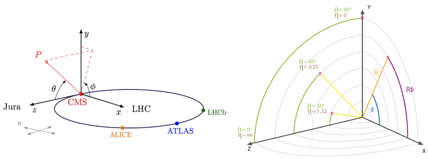
- the momentum transverse to the beam direction pt
- two angles θ (polar) and φ (azimuthal) - see picture below for the CMS reference frame used
- for convenience, at hadron colliders, the pseudorapidity η, defined as η =-ln(tan(η/2)) is used instead of the polar angle θ.
We will use some of them for training our Machine Learning algorithms.
How to execute it
Use Googe Colab
What is Google Colab?
Google's Colaboratory is a free online cloud-based Jupyter notebook environment on Google-hosted machines, with some added features, like the possibility to attach a GPU or a TPU if needed with 12 hours of continuous execution time. After that, the whole virtual machine is cleared and one has to start again. The user can run multiple CPU, GPU, and TPU instances simultaneously, but the resources are shared between these instances.
Open the Use Case Colab Notebook
The notebook for this tutorial can be found here. The .ipynb file is available in the attachment section and in this GitHub repository.
Indeed, the notebook can be opened by inserting the GitHub URL bdanzi/Higgs_exercise and clicking on the VBF_exercise.ipynb icon :

OR one can just click on the following link: https://colab.research.google.com/drive/1hVA0E5kosM2gdFkJINb6WeVp5hjG1ML1?usp=sharing.
Be sure to work on a copy of the notebook in Google Drive in both cases clicking on the Copy to Drive icon as shown below:
In order to do this, you must have a personal Google account.
Input files
The datasets files are stored on Recas Bari's ownCloud and are automatically loaded by the notebook. In case, they are also available here (4 muons decay channel) for the main exercise and here (4 electrons decay channel) for the optional exercise.
In the following, the most important excerpts are described.
Annotated Description
Load data using PANDAS data frames
Now you can start using your data and load three different NumPy arrays! One corresponds to the VBF signal and the other two will represent the Higgs boson production via the strong interaction processes (in jargon, QCD)
and
that will be used as a merged background.
Moreover, you will look at the physical observables that you can use to train the ML algorithms.
In [ ]:
#import libraries

import uproot
import numpy as np
import pandas as pd
import h5py
import seaborn as sns

from sklearn.utils import shuffle
from sklearn.model_selection import train_test_split
from sklearn.datasets import make_classification

import tensorflow as tf
from tensorflow import keras
from tensorflow.keras.models import Sequential, Model
from tensorflow.keras.optimizers import SGD, Adam, RMSprop, Adagrad, Adadelta
from tensorflow.keras.layers import Input, Activation, Dense, Dropout
from tensorflow.keras.callbacks import EarlyStopping, ReduceLROnPlateau, ModelCheckpoint
from tensorflow.keras import utils
from tensorflow import random as tf_random
from keras.utils import plot_model
import random as python_random
# Fix random seed for reproducibility

# The below is necessary for starting Numpy generated random numbers
# in a well-defined initial state.
seed = 7
np.random.seed(seed)

# The below is necessary for starting core Python generated random numbers
# in a well-defined state.
python_random.seed(seed)

# The below set_seed() will make random number generation
# in the TensorFlow backend have a well-defined initial state.
# For further details, see: https://www.tensorflow.org/api_docs/python/tf/random/set_seed
tf_random.set_seed(seed)

treename = 'HZZ4LeptonsAnalysisReduced'
filename = {}
upfile = {}
params = {}
df = {}

# Define what are the ROOT files we are interested in (for the two categories,
# signal and background)

filename['sig'] = 'VBF_HToZZTo4mu.root'
filename['bkg_ggHtoZZto4mu'] = 'GluGluHToZZTo4mu.root'
filename['bkg_ZZto4mu'] = 'ZZTo4mu.root'
#filename['bkg_ttH_HToZZ_4mu.root']= 'ttH_HToZZ_4mu.root'
#filename['sig'] = 'VBF_HToZZTo4e.root'
#filename['bkg_ggHtoZZto4e'] = 'GluGluHToZZTo4e.root'
#filename['bkg_ZZto4e'] = 'ZZTo4e.root'

# Variables from Root Tree that must be copyed to PANDA dataframe (df)
VARS = [ 'f_run', 'f_event', 'f_weight', \
        'f_massjj', 'f_deltajj', 'f_mass4l', 'f_Z1mass' , 'f_Z2mass', \
        'f_lept1_pt','f_lept1_eta','f_lept1_phi', \
        'f_lept2_pt','f_lept2_eta','f_lept2_phi', \
        'f_lept3_pt','f_lept3_eta','f_lept3_phi', \
        'f_lept4_pt','f_lept4_eta','f_lept4_phi', \
        'f_jet1_pt','f_jet1_eta','f_jet1_phi', \
        'f_jet2_pt','f_jet2_eta','f_jet2_phi' ]

#checking the dimensions of the df , 26 variables
NDIM = len(VARS)

print("Number of kinematic variables imported from the ROOT files = %d"% NDIM)

upfile['sig'] = uproot.open(filename['sig'])
upfile['bkg_ggHtoZZto4mu'] = uproot.open(filename['bkg_ggHtoZZto4mu'])
upfile['bkg_ZZto4mu'] = uproot.open(filename['bkg_ZZto4mu'])
#upfile['bkg_ttH_HToZZ_4mu.root'] = uproot.open(filename['bkg_ttH_HToZZ_4mu'])
#upfile['sig'] = uproot.open(filename['sig'])]
#upfile['bkg_ggHtoZZto4e'] = uproot.open(filename['bkg_ggHtoZZto4e'])
#upfile['bkg_ZZto4e'] = uproot.open(filename['bkg_ZZto4e'])
Number of kinematic variables imported from the ROOT files = 26
Let's see what you have uploaded in your Colab notebook!
# Look at the signal and bkg events before applying physical requirement

df['sig'] = pd.DataFrame(upfile['sig'][treename].arrays(VARS, library="np"),columns=VARS)
print(df['sig'].shape)
(24867, 26)
Comment: We have 24867 rows, i.e. 24867 different events, and 26 columns (whose meaning will be explained later).
Let's print out the first rows of this data set!
df['sig'].head()
| f_run | f_event | f_weight | f_massjj | f_deltajj | f_mass4l | f_Z1mass | f_Z2mass | f_lept1_pt | f_lept1_eta | f_lept1_phi | f_lept2_pt | f_lept2_eta | f_lept2_phi | f_lept3_pt | f_lept3_eta | f_lept3_phi | f_lept4_pt | f_lept4_eta | f_lept4_phi | f_jet1_pt | f_jet1_eta | f_jet1_phi | f_jet2_pt | f_jet2_eta | f_jet2_phi | |
|---|---|---|---|---|---|---|---|---|---|---|---|---|---|---|---|---|---|---|---|---|---|---|---|---|---|---|
| 0 | 1 | 385228 | 0.000176 | 667.271423 | 3.739947 | 124.966576 | 90.768616 | 20.508274 | 82.890457 | 0.822203 | 1.343706 | 65.486946 | 0.382922 | 2.568485 | 39.838531 | 0.546917 | 2.497204 | 28.562206 | 0.174666 | 2.013540 | 116.326035 | -1.126533 | -1.759238 | 90.333893 | 2.613415 | -0.096671 |
| 1 | 1 | 385233 | 0.000127 | 129.085892 | 0.046317 | 120.231926 | 80.782318 | 34.261726 | 41.195362 | -0.534245 | 2.802684 | 24.911942 | -2.065928 | 0.371150 | 21.959597 | -1.219900 | -2.938914 | 16.676077 | -0.162915 | 1.783374 | 105.491882 | 3.253374 | -1.297283 | 38.978493 | 3.207056 | 1.553476 |
| 2 | 1 | 385254 | 0.000037 | 285.165222 | 3.166899 | 125.254646 | 91.392693 | 25.695290 | 80.788002 | 0.943778 | 0.729632 | 35.549721 | 0.935241 | 1.288549 | 23.206284 | 0.236346 | -2.670540 | 14.581854 | 1.516623 | 0.284658 | 69.315170 | 2.573589 | -2.030811 | 51.972664 | -0.593310 | -2.799394 |
| 3 | 1 | 385260 | 0.000043 | 52.006794 | 0.150803 | 125.067009 | 91.183708 | 19.631315 | 129.883423 | 0.235406 | -1.729384 | 37.950790 | 1.226075 | -2.540356 | 17.678413 | 0.096546 | -1.533120 | 8.197763 | -0.157577 | 0.339215 | 202.689468 | 2.530802 | 1.325786 | 41.343758 | 2.681605 | 0.858582 |
| 4 | 1 | 385263 | 0.000092 | 1044.083496 | 4.315164 | 124.305748 | 72.480515 | 43.826504 | 86.220734 | -0.226653 | 0.117277 | 80.451378 | -0.536749 | 0.385678 | 27.497240 | 0.827591 | -0.072236 | 21.243813 | -0.579560 | -0.884727 | 127.192223 | -2.362456 | -2.945257 | 115.200272 | 1.952708 | 2.053301 |
The first 2 columns contain information which is provided by experiments at the LHC that will not be used in the training of our Machine Learning algorithms, therefore we skip our explanation to the next columns.
The next variable is the
f_weights. This corresponds to the probability of having that particular kind of physical process on the whole experiment. Indeed, it is a product of Branching Ratio (BR), geometrical acceptance of the detector, and kinematic phase-space. It is very important for the trainings phase and you will use it later.The variables
f_massjj,f_deltajj,f_mass4l,f_Z1mass, andf_Z2massare named high-level features (event features) since they contain overall information about the final-state particles (the mass of the two jets, their separation in space, the invariant mass of the four leptons, the masses of the two Z bosons). Note that themass is lighter w.r.t. the
one. Why is that? In the Higgs boson production (hypothesis of mass = 125 GeV) only one of the Z bosons is an actual particle that has the nominal mass of 91.18 GeV. The other one is a virtual (off-mass shell) particle.
The remnant columns represent the low-level features (object kinematics observables), the basic measurements which are made by the detectors for the individual final state objects (in our case four charged leptons and jets) such as
f_lept1(2,3,4)_pt(phi,eta)corresponding to their transverse momentum and the spatial distribution of their tracks ().
The same comments hold for the background datasets:
# Part of the code in "#" can be used in the second part of the exercise
# for trying to use alternative datasets for the training of our ML algorithms

#df['bkg'] = pd.DataFrame(upfile['bkg'][treename].arrays(VARS, library="np"),columns=VARS)
#df['bkg'].head()
df['bkg_ggHtoZZto4mu'] = pd.DataFrame(upfile['bkg_ggHtoZZto4mu'][treename].arrays(VARS, library="np"),columns=VARS)
df['bkg_ggHtoZZto4mu'].head()
#df['bkg_ggHtoZZto4e'] = pd.DataFrame(upfile['bkg_ggHtoZZto4e'][treename].arrays(VARS, library="np"),columns=VARS)
#df['bkg_ggHtoZZto4e'].head()
#df['bkg_ZZto4e'] = pd.DataFrame(upfile['bkg_ZZto4e'][treename].arrays(VARS, library="np"),columns=VARS)
#df['bkg_ZZto4e'].head()
Out[ ]:
| f_run | f_event | f_weight | f_massjj | f_deltajj | f_mass4l | f_Z1mass | f_Z2mass | f_lept1_pt | f_lept1_eta | f_lept1_phi | f_lept2_pt | f_lept2_eta | f_lept2_phi | f_lept3_pt | f_lept3_eta | f_lept3_phi | f_lept4_pt | f_lept4_eta | f_lept4_phi | f_jet1_pt | f_jet1_eta | f_jet1_phi | f_jet2_pt | f_jet2_eta | f_jet2_phi | |
|---|---|---|---|---|---|---|---|---|---|---|---|---|---|---|---|---|---|---|---|---|---|---|---|---|---|---|
| 0 | 1 | 581632 | 0.000225 | -999.0 | -999.0 | 120.101105 | 88.262352 | 22.051540 | 57.572330 | -0.433627 | -0.886073 | 56.933735 | 0.496556 | 0.404675 | 33.584896 | -0.037387 | 0.291866 | 10.881461 | -1.112960 | 0.051097 | 73.541260 | 1.683280 | 2.736636 | -999.0 | -999.0 | -999.0 |
| 1 | 1 | 581659 | 0.000277 | -999.0 | -999.0 | 124.592812 | 82.174683 | 17.613417 | 50.365120 | 0.001362 | 0.933713 | 31.548225 | 0.598417 | -1.863556 | 22.758055 | 0.220867 | -2.767246 | 17.264626 | 0.361964 | -1.859138 | -999.000000 | -999.000000 | -999.000000 | -999.0 | -999.0 | -999.0 |
| 2 | 1 | 581671 | 0.000278 | -999.0 | -999.0 | 125.692230 | 79.915764 | 29.998011 | 72.355927 | -0.238323 | -2.335623 | 20.644920 | -0.241560 | 1.855536 | 16.031651 | -1.446993 | 1.185016 | 11.068296 | 0.366903 | -0.606845 | 64.440544 | 1.886244 | 1.635723 | -999.0 | -999.0 | -999.0 |
| 3 | 1 | 581724 | 0.000336 | -999.0 | -999.0 | 125.027504 | 85.200958 | 23.440151 | 43.059235 | 0.759979 | -1.714778 | 19.248983 | 0.535979 | 0.420337 | 16.595169 | -1.330326 | 1.656061 | 11.407483 | -0.686118 | 1.295116 | -999.000000 | -999.000000 | -999.000000 | -999.0 | -999.0 | -999.0 |
| 4 | 1 | 581744 | 0.000273 | -999.0 | -999.0 | 124.917282 | 65.971390 | 14.968305 | 52.585011 | -0.656421 | -2.933651 | 35.095982 | -1.002568 | 0.865173 | 28.146715 | -0.730926 | -0.876442 | 8.034222 | -1.094436 | 1.783626 | -999.000000 |
df['bkg_ZZto4mu'] = pd.DataFrame(upfile['bkg_ZZto4mu'][treename].arrays(VARS, library="np"),columns=VARS)
df['bkg_ZZto4mu'].head()
| f_run | f_event | f_weight | f_massjj | f_deltajj | f_mass4l | f_Z1mass | f_Z2mass | f_lept1_pt | f_lept1_eta | f_lept1_phi | f_lept2_pt | f_lept2_eta | f_lept2_phi | f_lept3_pt | f_lept3_eta | f_lept3_phi | f_lept4_pt | f_lept4_eta | f_lept4_phi | f_jet1_pt | f_jet1_eta | f_jet1_phi | f_jet2_pt | f_jet2_eta | f_jet2_phi | |
|---|---|---|---|---|---|---|---|---|---|---|---|---|---|---|---|---|---|---|---|---|---|---|---|---|---|---|
| 0 | 1 | 1991117 | 0.001420 | 384.394165 | 0.235409 | 309.921478 | 93.538399 | 87.436043 | 84.918190 | -0.073681 | -1.339234 | 60.143539 | -1.229701 | -1.409149 | 54.892681 | 1.125339 | -1.046433 | 42.139397 | 0.966109 | 2.593184 | 240.828506 | 0.103300 | 2.408482 | 195.838226 | 0.338708 | 0.285348 |
| 1 | 1 | 1991192 | 0.000893 | 110.589844 | 0.956070 | 326.481903 | 92.948936 | 85.379288 | 124.270218 | 1.388811 | -1.738097 | 87.379723 | 0.766540 | 2.502843 | 54.472603 | -0.106614 | 1.626933 | 18.505959 | 2.012172 | 2.229677 | 77.210411 | 2.061765 | -0.532572 | 48.432365 | 1.105695 | 1.128457 |
| 2 | 1 | 1991331 | 0.000839 | -999.000000 | -999.000000 | 91.167046 | 56.161217 | 14.535084 | 25.241573 | 1.410529 | 2.080089 | 21.971258 | 1.465800 | 1.868505 | 20.648312 | 0.787121 | 2.017863 | 9.831321 | -1.329539 | 2.286600 | 66.642792 | 1.176917 | -1.089489 | -999.000000 | -999.000000 | -999.000000 |
| 3 | 1 | 1991364 | 0.000906 | -999.000000 | -999.000000 | 323.428345 | 88.717270 | 94.940346 | 65.728729 | -0.561113 | 2.596448 | 50.528595 | 2.227971 | 0.101310 | 39.392380 | 0.294608 | -1.756674 | 33.169487 | 0.367907 | -0.241346 | -999.000000 | -999.000000 | -999.000000 | -999.000000 | -999.000000 | -999.000000 |
| 4 | 1 | 1991360 | 0.001034 | -999.000000 | -999.000000 | 274.207916 | 90.799271 | 90.156898 | 101.931305 | 0.828778 | 2.440133 | 89.171135 | -0.052834 |
# Let's merge our background processes together!
df['bkg'] = pd.concat([df['bkg_ZZto4mu'],df['bkg_ggHtoZZto4mu']])
# Let's shuffle them!
df['bkg']= shuffle(df['bkg'])
# Let's see its shape!
print(df['bkg'].shape)
#print(len(df['bkg']))
#print(len(df['bkg_ZZto4mu']))
#print(len(df['bkg_ggHtoZZto4mu']))
#print(len(df['bkg_ggHtoZZto4e']))
#print(len(df['bkg_ZZto4e']))
(952342, 26)
Note that the background datasets seem to have a very large number of events! Is that true? Do all physical variables have meaningful values? Let's make physical selection requirements!
# Remove undefined variable entries VARS[i] <= -999

for i in range(NDIM):
    df['sig'] = df['sig'][(df['sig'][VARS[i]] > -999)]
    df['bkg']= df['bkg'][(df['bkg'][VARS[i]] > -999)]

# Add the columnisSignal to the dataframe containing the truth information
# i.e. it tells if that particular event is signal (isSignal=1) or background (isSignal=0)

df['sig']['isSignal'] = np.ones(len(df['sig']))
df['bkg']['isSignal'] = np.zeros(len(df['bkg']))
print("Number of Signal events = %d " %len(df['sig']['isSignal']))
print("Number of Background events = %d " %len(df['bkg']['isSignal']))
Number of Signal events = 14260
Number of Background events = 100724
#Showing that the variable isSignal is correctly assigned for VBF signal events
print(df['sig']['isSignal'])
0        1.0
1        1.0
2        1.0
3        1.0
4        1.0
        ...
24858    1.0
24859    1.0
24860    1.0
24861    1.0
24862    1.0
Name: isSignal, Length: 14260, dtype: float64
# Showing that the variable isSignal is correctly assigned for bkg events
# Some events are missing because of the selection. So we do not have in total 134682
# background events anymore!
print(df['bkg']['isSignal'])
42646     0.0
619246    0.0
360856    0.0
727095    0.0
8984      0.0
         ...
551642    0.0
315737    0.0
759363    0.0
535030    0.0
189636    0.0
Name: isSignal, Length: 100724, dtype: float64
Let's see in which way we have to use the f_weight variable!
# Renormalizes the events weights to give unit sum in the signal and background dataframes
# This is necessary for the ML algorithms to learn signal and background
# in the same proportion,independently of number of events
# and absolute weights of events in each sample of events!
# The relative contributions of each background process is retained - so the classifier
# learns to focus more on the importance backgrounds, and the background matches the data
# shape - but overall signal and background have equal importance (the classifier
# learns to identify signal and background equally well).
# In the pandas technical vocabolary axis=0 stands for columns, axis=1 for rows.

df['sig']['f_weight']=df['sig']['f_weight']/df['sig']['f_weight'].sum(axis=0)
df['bkg']['f_weight']=df['bkg']['f_weight']/df['bkg']['f_weight'].sum(axis=0)

# Note: Number of events remain unchanged after this "normalization procedure"
print("Number SIG events=", len(df['sig']['f_weight']))
print("Number BKG events=", len(df['bkg']['f_weight']))
Number SIG events= 14260
Number BKG events= 100724
Let's merge our signal and background events!
# Concatenate the signal and background dfs in a single data frame
df_all = pd.concat([df['sig'],df['bkg']])

# Random shuffles the data set to mix signal and background events
# before the splitting between train and test datasets
df_all = shuffle(df_all)
Preparing input features for the ML algorithms
We have our data set ready to train our ML algorithms! Before doing that we have to decide from which input variables the computer algorithms have to learn to distinguish between signal and background events.
We can use:
- The five high-level input variables
f_massjj,f_deltajj,f_mass4l,f_Z1mass, andf_Z2mass. - The 18 kinematic variables characterize the four-lepton + two jest final states objects.
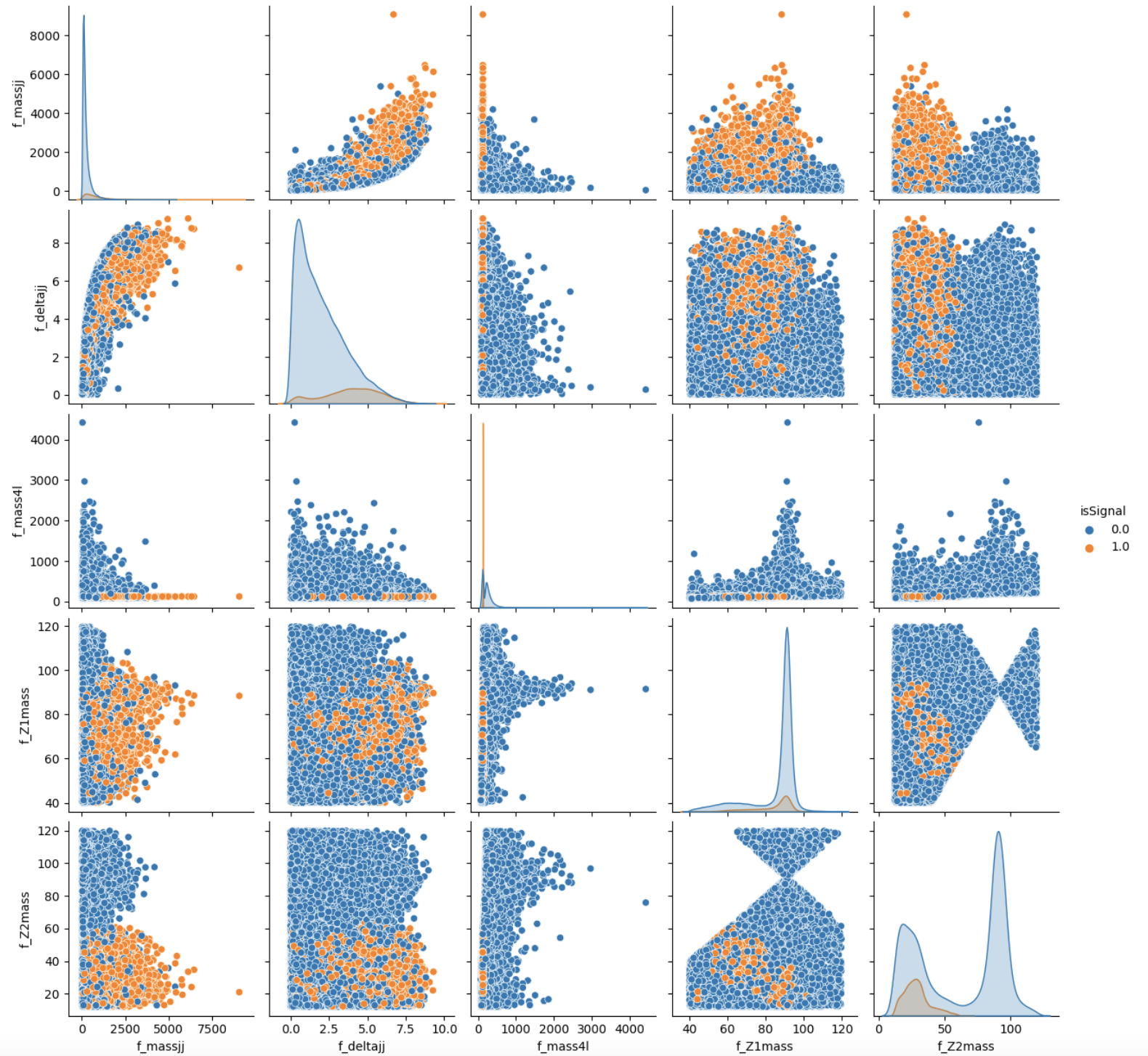
To make this choice, we can look at the two sets of correlation plots - the so-called scatter plots using the seaborn library - among the features at our disposal and see which set captures better the differences between signal and background events.
Note: this operation is quite long for both sets since we are dealing with quite a lot of events. Skip the following two code cells and trust us in using the high-level features for building your ML models! Indeed, we will obtain better discriminators' performance using high-level features. You can always return to this part of the exercise and try to use the low-level features.
# It will take a while (5 minutes), you can skip it as said before.
# We leave you the output of this code cell using a .png format
# VAR = [ 'f_massjj', 'f_deltajj', 'f_mass4l', 'f_Z1mass' , 'f_Z2mass', 'isSignal']
# sns.pairplot( data=df_all.filter(VAR), hue='isSignal' , kind='scatter', diag_kind='auto' );
# It will take a while (1 hour). Skip it!
# We leave you the output of this code cell using a .png format

# NN_VARS = ['f_lept1_pt','f_lept1_eta','f_lept1_phi', \
#           'f_lept2_pt','f_lept2_eta','f_lept2_phi', \
#           'f_lept3_pt','f_lept3_eta','f_lept3_phi', \
#           'f_lept4_pt','f_lept4_eta','f_lept4_phi', \
#           'f_jet1_pt','f_jet1_eta','f_jet1_phi', \
#           'f_jet2_pt','f_jet2_eta','f_jet2_phi', 'isSignal']
# sns.pairplot( data=df_all.filter(NN_VARS), hue='isSignal' , kind='scatter', diag_kind='auto' );